ARFS - How to use with large data?#
It might be than the data set is too large for All Relevant Feature Selection to run in a reasonable time. Usually random sampling (stratified, grouped, etc) solves this issues. If extreme sampling is needed, ARFS provide two methods for decreasing drastically the number of rows. The sampling methods and outcomes are illustrated below.
[18]:
# from IPython.core.display import display, HTML
# display(HTML("<style>.container { width:95% !important; }</style>"))
import numpy as np
import pandas as pd
import matplotlib.pyplot as plt
import gc

from sklearn.pipeline import Pipeline

import arfs.feature_selection as arfsfs
from arfs.preprocessing import OrdinalEncoderPandas
from arfs.benchmark import highlight_tick, compare_varimp, sklearn_pimp_bench
from arfs.utils import load_data
from arfs.sampling import sample

# plt.style.use('fivethirtyeight')
rng = np.random.RandomState(seed=42)

import warnings

warnings.filterwarnings("ignore")
[2]:
import arfs

print(f"Run with ARFS {arfs.__version__}")
Run with ARFS 3.0.0
[3]:
%matplotlib inline
[4]:
gc.enable()
gc.collect()
[4]:
4
Sampling data#
A fairly large data set for illustration
[5]:
# X, y, w = _generated_corr_dataset_regr(size=100_000)

housing = load_data(name="housing")
X, y = housing.data, housing.target

X = pd.DataFrame(X)
X.columns = housing.feature_names
y = pd.Series(y)
X.head()
[5]:
| MedInc | HouseAge | AveRooms | AveBedrms | Population | AveOccup | Latitude | Longitude | |
|---|---|---|---|---|---|---|---|---|
| 0 | 8.3252 | 41.0 | 6.984127 | 1.023810 | 322.0 | 2.555556 | 37.88 | -122.23 |
| 1 | 8.3014 | 21.0 | 6.238137 | 0.971880 | 2401.0 | 2.109842 | 37.86 | -122.22 |
| 2 | 7.2574 | 52.0 | 8.288136 | 1.073446 | 496.0 | 2.802260 | 37.85 | -122.24 |
| 3 | 5.6431 | 52.0 | 5.817352 | 1.073059 | 558.0 | 2.547945 | 37.85 | -122.25 |
| 4 | 3.8462 | 52.0 | 6.281853 | 1.081081 | 565.0 | 2.181467 | 37.85 | -122.25 |
Cleaning the data#
[6]:
basic_fs_pipeline = Pipeline(
[
("missing", arfsfs.MissingValueThreshold(threshold=0.05)),
("unique", arfsfs.UniqueValuesThreshold(threshold=1)),
("cardinality", arfsfs.CardinalityThreshold(threshold=10)),
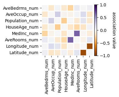
("collinearity", arfsfs.CollinearityThreshold(threshold=0.75)),
]
)
X_trans = basic_fs_pipeline.fit_transform(X=X, y=y)
# collinearity__sample_weight=w,
# lowimp__sample_weight=w)
[7]:
f = basic_fs_pipeline.named_steps["collinearity"].plot_association(figsize=(4, 4))
[8]:
data = X_trans.copy()
data["target"] = y.values
[9]:
print(f"The dataset shape is {data.shape}")
The dataset shape is (20640, 8)
Random sampling#
You can sample using pandas or scikit-learn (providing more advanced random sampling, as stratified sampling, depending on the task).
[10]:
data_rnd_samp = data.sample(n=1_000)
print(f"The sampled dataset shape is {data_rnd_samp.shape}")
The sampled dataset shape is (1000, 8)
Sampling by clustering the rows#
Using the Gower distance (handling mixed-type data), the rows are clustered and the average/mode for each column is returned. The larger the number of clusters, the closer to the original data. As it requires the computation of a distance matrix, you might need to use random sampling first to avoid a computational bottleneck.
[ ]:
%%time
data_dum = data.sample(n=10_000)
data_dum = data.copy()
# Compute a distance matrix, 10_000x10_000 and use it for clustering (1_000 clusters)
data_g_samp = sample(df=data_dum, n=1_000, sample_weight=None, method="gower")
print(f"The sampled dataset shape is {data_g_samp.shape}")
Sampling by removing outliers#
This method is adapted from BorutaShap. It uses IsolationForest to remove the less similar samples and iterates till the 2-sample KS statistics is > \(95\%\) (for having a similar distribution than the original data). There is no guarantee of the output size.
[11]:
%%time
data_isof_samp = sample(df=data, sample_weight=None, method="isoforest")
print(f"The sampled dataset shape is {data_isof_samp.shape}")
The sampled dataset shape is (2064, 8)
CPU times: user 604 ms, sys: 7.84 ms, total: 612 ms
Wall time: 711 ms
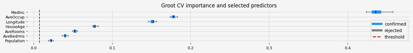
Impact on the feature selection#
Let’s perform the feature selection on this toy data set to see what is the impact of the different sampling strategies.
[16]:
%%time
# No Sampling
X = data.drop("target", axis=1)
y = data.target

# GrootCV
feat_selector = arfsfs.GrootCV(
    objective="rmse", cutoff=1, n_folds=5, n_iter=5, silent=True
)
feat_selector.fit(X, y, sample_weight=None)
print(feat_selector.get_feature_names_out())
fig = feat_selector.plot_importance(n_feat_per_inch=5)

# highlight synthetic random variable
fig = highlight_tick(figure=fig, str_match="random")
fig = highlight_tick(figure=fig, str_match="genuine", color="green")
plt.show()
Training until validation scores don't improve for 20 rounds
Early stopping, best iteration is:
[151]   training's l2: 0.204331     valid_1's l2: 0.326671
Training until validation scores don't improve for 20 rounds
Early stopping, best iteration is:
[95]    training's l2: 0.240687     valid_1's l2: 0.312489
Training until validation scores don't improve for 20 rounds
Early stopping, best iteration is:
[219]   training's l2: 0.175836     valid_1's l2: 0.346323
Training until validation scores don't improve for 20 rounds
Early stopping, best iteration is:
[117]   training's l2: 0.228562     valid_1's l2: 0.303057
Training until validation scores don't improve for 20 rounds
Early stopping, best iteration is:
[77]    training's l2: 0.251179     valid_1's l2: 0.337232
Training until validation scores don't improve for 20 rounds
Early stopping, best iteration is:
[125]   training's l2: 0.221841     valid_1's l2: 0.316486
Training until validation scores don't improve for 20 rounds
Early stopping, best iteration is:
[122]   training's l2: 0.223227     valid_1's l2: 0.334787
Training until validation scores don't improve for 20 rounds
Early stopping, best iteration is:
[162]   training's l2: 0.199937     valid_1's l2: 0.320165
Training until validation scores don't improve for 20 rounds
Early stopping, best iteration is:
[145]   training's l2: 0.207626     valid_1's l2: 0.325318
Training until validation scores don't improve for 20 rounds
Early stopping, best iteration is:
[156]   training's l2: 0.203951     valid_1's l2: 0.335031
Training until validation scores don't improve for 20 rounds
Early stopping, best iteration is:
[137]   training's l2: 0.213178     valid_1's l2: 0.34583
Training until validation scores don't improve for 20 rounds
Early stopping, best iteration is:
[129]   training's l2: 0.218581     valid_1's l2: 0.315213
Training until validation scores don't improve for 20 rounds
Early stopping, best iteration is:
[122]   training's l2: 0.218357     valid_1's l2: 0.336374
Training until validation scores don't improve for 20 rounds
Early stopping, best iteration is:
[111]   training's l2: 0.232967     valid_1's l2: 0.313847
Training until validation scores don't improve for 20 rounds
Early stopping, best iteration is:
[145]   training's l2: 0.20741      valid_1's l2: 0.322324
Training until validation scores don't improve for 20 rounds
Early stopping, best iteration is:
[100]   training's l2: 0.23626      valid_1's l2: 0.309587
Training until validation scores don't improve for 20 rounds
Early stopping, best iteration is:
[167]   training's l2: 0.196718     valid_1's l2: 0.336912
Training until validation scores don't improve for 20 rounds
Early stopping, best iteration is:
[185]   training's l2: 0.187894     valid_1's l2: 0.333857
Training until validation scores don't improve for 20 rounds
Early stopping, best iteration is:
[170]   training's l2: 0.19827      valid_1's l2: 0.319529
Training until validation scores don't improve for 20 rounds
Early stopping, best iteration is:
[168]   training's l2: 0.193972     valid_1's l2: 0.329542
Training until validation scores don't improve for 20 rounds
Early stopping, best iteration is:
[141]   training's l2: 0.209756     valid_1's l2: 0.340815
Training until validation scores don't improve for 20 rounds
Early stopping, best iteration is:
[116]   training's l2: 0.225559     valid_1's l2: 0.322635
Training until validation scores don't improve for 20 rounds
Early stopping, best iteration is:
[76]    training's l2: 0.253261     valid_1's l2: 0.328681
Training until validation scores don't improve for 20 rounds
Early stopping, best iteration is:
[151]   training's l2: 0.208201     valid_1's l2: 0.320702
Training until validation scores don't improve for 20 rounds
Early stopping, best iteration is:
[100]   training's l2: 0.235078     valid_1's l2: 0.31675
['MedInc' 'HouseAge' 'AveRooms' 'AveBedrms' 'Population' 'AveOccup'
 'Longitude']
---------------------------------------------------------------------------
NameError                                 Traceback (most recent call last)
File <timed exec>:14

NameError: name 'highlight_tick' is not defined
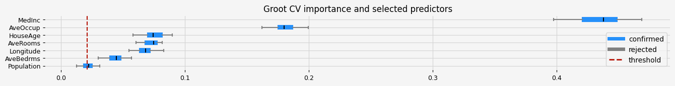
[17]:
%%time

X = data_rnd_samp.drop("target", axis=1)
y = data_rnd_samp.target

# GrootCV
feat_selector = arfsfs.GrootCV(
    objective="rmse", cutoff=1, n_folds=5, n_iter=5, silent=True
)
feat_selector.fit(X, y, sample_weight=None)
print(feat_selector.get_feature_names_out())
fig = feat_selector.plot_importance(n_feat_per_inch=5)

# highlight synthetic random variable
fig = highlight_tick(figure=fig, str_match="random")
fig = highlight_tick(figure=fig, str_match="genuine", color="green")
plt.show()
Training until validation scores don't improve for 20 rounds
Early stopping, best iteration is:
[30]    training's l2: 0.166799     valid_1's l2: 0.375475
Training until validation scores don't improve for 20 rounds
Early stopping, best iteration is:
[45]    training's l2: 0.0961632    valid_1's l2: 0.470772
Training until validation scores don't improve for 20 rounds
Early stopping, best iteration is:
[52]    training's l2: 0.0891238    valid_1's l2: 0.486354
Training until validation scores don't improve for 20 rounds
Early stopping, best iteration is:
[32]    training's l2: 0.167216     valid_1's l2: 0.376773
Training until validation scores don't improve for 20 rounds
Early stopping, best iteration is:
[46]    training's l2: 0.0968427    valid_1's l2: 0.431018
Training until validation scores don't improve for 20 rounds
Early stopping, best iteration is:
[41]    training's l2: 0.119891     valid_1's l2: 0.359728
Training until validation scores don't improve for 20 rounds
Early stopping, best iteration is:
[60]    training's l2: 0.0684558    valid_1's l2: 0.449729
Training until validation scores don't improve for 20 rounds
Early stopping, best iteration is:
[43]    training's l2: 0.100557     valid_1's l2: 0.374715
Training until validation scores don't improve for 20 rounds
Early stopping, best iteration is:
[45]    training's l2: 0.0956372    valid_1's l2: 0.469351
Training until validation scores don't improve for 20 rounds
Early stopping, best iteration is:
[32]    training's l2: 0.134747     valid_1's l2: 0.547114
Training until validation scores don't improve for 20 rounds
Early stopping, best iteration is:
[33]    training's l2: 0.15071      valid_1's l2: 0.397982
Training until validation scores don't improve for 20 rounds
Early stopping, best iteration is:
[29]    training's l2: 0.176599     valid_1's l2: 0.421348
Training until validation scores don't improve for 20 rounds
Early stopping, best iteration is:
[25]    training's l2: 0.193759     valid_1's l2: 0.444774
Training until validation scores don't improve for 20 rounds
Early stopping, best iteration is:
[33]    training's l2: 0.147421     valid_1's l2: 0.500831
Training until validation scores don't improve for 20 rounds
Early stopping, best iteration is:
[48]    training's l2: 0.0932204    valid_1's l2: 0.404222
Training until validation scores don't improve for 20 rounds
Early stopping, best iteration is:
[67]    training's l2: 0.0487236    valid_1's l2: 0.506928
Training until validation scores don't improve for 20 rounds
Early stopping, best iteration is:
[37]    training's l2: 0.128301     valid_1's l2: 0.442707
Training until validation scores don't improve for 20 rounds
Early stopping, best iteration is:
[45]    training's l2: 0.0989439    valid_1's l2: 0.42606
Training until validation scores don't improve for 20 rounds
Early stopping, best iteration is:
[63]    training's l2: 0.0657157    valid_1's l2: 0.432651
Training until validation scores don't improve for 20 rounds
Early stopping, best iteration is:
[57]    training's l2: 0.068082     valid_1's l2: 0.408432
Training until validation scores don't improve for 20 rounds
Early stopping, best iteration is:
[57]    training's l2: 0.068025     valid_1's l2: 0.499865
Training until validation scores don't improve for 20 rounds
Early stopping, best iteration is:
[37]    training's l2: 0.126191     valid_1's l2: 0.419695
Training until validation scores don't improve for 20 rounds
Early stopping, best iteration is:
[29]    training's l2: 0.16468      valid_1's l2: 0.419023
Training until validation scores don't improve for 20 rounds
Early stopping, best iteration is:
[34]    training's l2: 0.144042     valid_1's l2: 0.430156
Training until validation scores don't improve for 20 rounds
Early stopping, best iteration is:
[45]    training's l2: 0.102332     valid_1's l2: 0.463595
['MedInc' 'HouseAge' 'AveRooms' 'AveBedrms' 'Population' 'AveOccup'
 'Longitude']
---------------------------------------------------------------------------
NameError                                 Traceback (most recent call last)
File <timed exec>:13

NameError: name 'highlight_tick' is not defined
[19]:
%%time

X = data_g_samp.drop("target", axis=1)
y = data_g_samp.target

# GrootCV
feat_selector = arfsfs.GrootCV(
    objective="rmse", cutoff=1, n_folds=5, n_iter=5, silent=True
)
feat_selector.fit(X, y, sample_weight=None)
print(feat_selector.get_feature_names_out())
fig = feat_selector.plot_importance(n_feat_per_inch=5)

# highlight synthetic random variable
fig = highlight_tick(figure=fig, str_match="random")
fig = highlight_tick(figure=fig, str_match="genuine", color="green")
plt.show()
---------------------------------------------------------------------------
NameError                                 Traceback (most recent call last)
File <timed exec>:1

NameError: name 'data_g_samp' is not defined
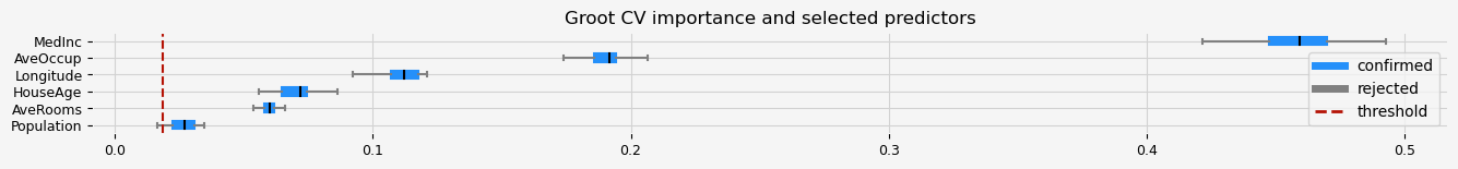
[21]:
%%time

X = data_isof_samp.drop("target", axis=1)
y = data_isof_samp.target

# GrootCV
feat_selector = arfsfs.GrootCV(
    objective="rmse", cutoff=1, n_folds=5, n_iter=5, silent=True
)
feat_selector.fit(X, y, sample_weight=None)
print(feat_selector.get_feature_names_out())
fig = feat_selector.plot_importance(n_feat_per_inch=5)

# highlight synthetic random variable
fig = highlight_tick(figure=fig, str_match="random")
fig = highlight_tick(figure=fig, str_match="genuine", color="green")
plt.show()
Training until validation scores don't improve for 20 rounds
Early stopping, best iteration is:
[41]    training's l2: 0.143895     valid_1's l2: 0.419566
Training until validation scores don't improve for 20 rounds
Early stopping, best iteration is:
[49]    training's l2: 0.123278     valid_1's l2: 0.397813
Training until validation scores don't improve for 20 rounds
Early stopping, best iteration is:
[37]    training's l2: 0.159719     valid_1's l2: 0.383639
Training until validation scores don't improve for 20 rounds
Early stopping, best iteration is:
[56]    training's l2: 0.11299      valid_1's l2: 0.366118
Training until validation scores don't improve for 20 rounds
Early stopping, best iteration is:
[66]    training's l2: 0.0896061    valid_1's l2: 0.397312
Training until validation scores don't improve for 20 rounds
Early stopping, best iteration is:
[39]    training's l2: 0.157648     valid_1's l2: 0.373146
Training until validation scores don't improve for 20 rounds
Early stopping, best iteration is:
[50]    training's l2: 0.123834     valid_1's l2: 0.39308
Training until validation scores don't improve for 20 rounds
Early stopping, best iteration is:
[40]    training's l2: 0.159366     valid_1's l2: 0.316867
Training until validation scores don't improve for 20 rounds
Early stopping, best iteration is:
[52]    training's l2: 0.114191     valid_1's l2: 0.457971
Training until validation scores don't improve for 20 rounds
Early stopping, best iteration is:
[46]    training's l2: 0.129243     valid_1's l2: 0.441562
Training until validation scores don't improve for 20 rounds
Early stopping, best iteration is:
[56]    training's l2: 0.10658      valid_1's l2: 0.358745
Training until validation scores don't improve for 20 rounds
Early stopping, best iteration is:
[48]    training's l2: 0.120558     valid_1's l2: 0.439188
Training until validation scores don't improve for 20 rounds
Early stopping, best iteration is:
[37]    training's l2: 0.161763     valid_1's l2: 0.397943
Training until validation scores don't improve for 20 rounds
Early stopping, best iteration is:
[43]    training's l2: 0.139222     valid_1's l2: 0.394755
Training until validation scores don't improve for 20 rounds
Early stopping, best iteration is:
[39]    training's l2: 0.153084     valid_1's l2: 0.405815
Training until validation scores don't improve for 20 rounds
Early stopping, best iteration is:
[48]    training's l2: 0.123297     valid_1's l2: 0.423094
Training until validation scores don't improve for 20 rounds
Early stopping, best iteration is:
[41]    training's l2: 0.155462     valid_1's l2: 0.341056
Training until validation scores don't improve for 20 rounds
Early stopping, best iteration is:
[31]    training's l2: 0.186186     valid_1's l2: 0.387608
Training until validation scores don't improve for 20 rounds
Early stopping, best iteration is:
[38]    training's l2: 0.161008     valid_1's l2: 0.386238
Training until validation scores don't improve for 20 rounds
Early stopping, best iteration is:
[41]    training's l2: 0.146398     valid_1's l2: 0.435355
Training until validation scores don't improve for 20 rounds
Early stopping, best iteration is:
[36]    training's l2: 0.161081     valid_1's l2: 0.469358
Training until validation scores don't improve for 20 rounds
Early stopping, best iteration is:
[32]    training's l2: 0.182545     valid_1's l2: 0.380976
Training until validation scores don't improve for 20 rounds
Early stopping, best iteration is:
[40]    training's l2: 0.151907     valid_1's l2: 0.364813
Training until validation scores don't improve for 20 rounds
Early stopping, best iteration is:
[38]    training's l2: 0.160105     valid_1's l2: 0.381487
Training until validation scores don't improve for 20 rounds
Early stopping, best iteration is:
[70]    training's l2: 0.0845652    valid_1's l2: 0.414601
['MedInc' 'HouseAge' 'AveRooms' 'AveBedrms' 'Population' 'AveOccup'
 'Longitude']
CPU times: user 43.9 s, sys: 736 ms, total: 44.6 s
Wall time: 15.7 s