Lasso Regularized GLM for Feature Selection in Python#
Introduction#
Welcome to our tutorial on using the Lasso Regularized Generalized Linear Model (GLM) for feature selection in Python! Feature selection is a critical step in machine learning, helping us identify the most important variables from a dataset, making models more accurate and easier to understand.
Description#
The Lasso Regularized GLM is a powerful variant of the traditional GLM. It adds a unique twist - the L1 regularization penalty (Lasso regularization). This penalty encourages some coefficients to become exactly zero, effectively excluding irrelevant features from the model. As a result, the Lasso Regularized GLM becomes an excellent tool for feature selection, especially in datasets with many variables.
In this tutorial, we’ll build a user-friendly Python class called “LassoFeatureSelection” that harnesses the Lasso Regularized GLM to perform feature selection. The class can handle different types of data, like pandas DataFrames and numpy arrays, making it super flexible and compatible with various data formats.
Please note that one limitation of the lasso is that it treats the levels of a categorical predictor individually. However, this issue can be addressed by utilizing the TreeDiscretizer, which automatically bins numerical variables and groups the levels of categorical variables.
Key Features of the “LassoFeatureSelection” Class#
Automated Intercept Handling: Our class automatically adds an intercept column to the input data if it’s missing. It then checks if the intercept is statistically significant and keeps it only if necessary.
Model Selection: We use a grid search cross-validation approach to find the best regularization parameter (alpha) for the Lasso Regularized GLM. Users can choose from two scoring options: the Bayesian Information Criterion (BIC) or the mean cross-validation score (deviance). The BIC is much faster.
Transparent Feature Selection: After fitting the “LassoFeatureSelection” model, you can access the selected features. This lets you understand which variables are the most crucial in the final model.
[2]:
import pandas as pd
import numpy as np
import matplotlib.pyplot as plt
import matplotlib

from mpl_toolkits.axes_grid1.inset_locator import inset_axes

from sklearn.datasets import make_regression
from sklearn.model_selection import train_test_split
from sklearn.preprocessing import StandardScaler
from sklearn.pipeline import Pipeline
from sklearn.linear_model import LinearRegression
from sklearn.linear_model import PoissonRegressor
from sklearn.metrics import mean_squared_error

from arfs.feature_selection.lasso import LassoFeatureSelection
from arfs.preprocessing import PatsyTransformer
import arfs.feature_selection as arfsfs


def plot_y_vs_X(
    X: pd.DataFrame, y: pd.Series, ncols: int = 2, figsize: tuple = (10, 10)
) -> plt.Figure:
    """
    Create subplots of scatter plots showing the relationship between each column in X and the target variable y.

    Parameters
    ----------
        X : pd.DataFrame
            The input DataFrame containing the predictor variables.
        y : pd.Series
            The target variable to be plotted against.
        ncols : int, optional (default: 2)
            The number of columns in the subplot grid.
        figsize : tuple, optional (default: (10, 10))
            The size of the figure (width, height) in inches.

    Returns
    -------
        plt.Figure
            The generated Figure object containing the scatter plots.
    """

    n_rows, ncols_to_plot = divmod(X.shape[1], ncols)
    n_rows += int(ncols_to_plot > 0)

    # Create figure and axes
    f, axs = plt.subplots(nrows=n_rows, ncols=ncols, figsize=figsize)

    # Iterate through columns and plot against y
    for ax, col in zip(axs.flat, X.columns):
        ax.scatter(X[col], y, alpha=0.1)
        ax.set_title(col)

    # Remove any unused subplots
    for ax in axs.flat[len(X.columns) :]:
        ax.set_axis_off()

    # Display the figure
    plt.tight_layout()
    return f
Linear model#
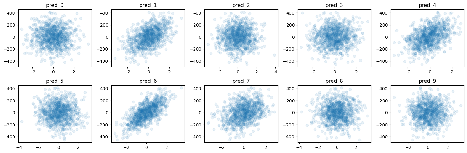
The main goal here is not to build a detailed model for the data, but rather to identify the most important predictors. We will check how well the feature selection process can distinguish between meaningful predictors and random noise.
[3]:
bias = 7.0
X, y, true_coef = make_regression(
    n_samples=2_000,
    n_features=10,
    n_informative=5,
    noise=1,
    random_state=8,
    bias=bias,
    coef=True,
)
X = pd.DataFrame(X)
X.columns = [f"pred_{i}" for i in range(X.shape[1])]

X_train, X_test, y_train, y_test = train_test_split(
    X, y, test_size=0.5, random_state=42
)

print(f"The true coefficient of the linear data generating process are:\n {true_coef}")
f = plot_y_vs_X(X_train, y_train, ncols=5, figsize=(15, 5))
The true coefficient of the linear data generating process are:
 [ 0.         77.90364383  0.          0.         63.70230035  0.
 95.59499715 43.86990345  0.          4.11861919]
[4]:
# family should be: "gaussian", "poisson", "gamma", "negativebinomial", "binomial", "tweedie"
selector = LassoFeatureSelection(n_iterations=10, family="gaussian", score="bic")
selector.fit(X=X_train, y=y_train, sample_weight=None)
selector.get_feature_names_out()
/home/bsatom/Documents/arfs_test_nbs/arfsuv/lib/python3.12/site-packages/sklearn/utils/deprecation.py:151: FutureWarning: 'force_all_finite' was renamed to 'ensure_all_finite' in 1.6 and will be removed in 1.8.
  warnings.warn(
[4]:
Index(['Intercept', 'pred_1', 'pred_4', 'pred_6', 'pred_7', 'pred_9'], dtype='object')
[5]:
true_coef = pd.Series(true_coef)
true_coef.index = X.columns
true_coef = pd.Series({**{"intercept": bias}, **true_coef})
true_coef
[5]:
intercept     7.000000
pred_0        0.000000
pred_1       77.903644
pred_2        0.000000
pred_3        0.000000
pred_4       63.702300
pred_5        0.000000
pred_6       95.594997
pred_7       43.869903
pred_8        0.000000
pred_9        4.118619
dtype: float64
[6]:
selector.transform(X_test).head()
[6]:
| Intercept | pred_1 | pred_4 | pred_6 | pred_7 | pred_9 | |
|---|---|---|---|---|---|---|
| 1860 | 1.0 | 1.091750 | -0.015868 | 0.231947 | -0.998250 | 0.041597 |
| 353 | 1.0 | -0.871767 | 2.557578 | -0.026118 | 0.936062 | 0.533048 |
| 1333 | 1.0 | 1.147664 | 0.678622 | -0.313260 | -1.717187 | 0.228773 |
| 905 | 1.0 | 2.247261 | -0.008657 | 0.354843 | 0.151635 | 2.047569 |
| 1289 | 1.0 | -0.061458 | -1.429949 | -1.012678 | -1.070863 | 0.768713 |
[7]:
selector.feature_names_in_
[7]:
Index(['Intercept', 'pred_0', 'pred_1', 'pred_2', 'pred_3', 'pred_4', 'pred_5',
       'pred_6', 'pred_7', 'pred_8', 'pred_9'],
      dtype='object')
[8]:
selector.support_
[8]:
array([ True, False,  True, False, False,  True, False,  True,  True,
       False,  True])
The exciting part is that lasso, despite potential mismatches in the distribution, can still perform remarkably well. It means that even if the data does not perfectly follow a certain pattern, lasso might successfully identify relevant predictors and filter out irrelevant ones.
[9]:
selector.get_feature_names_out()
[9]:
Index(['Intercept', 'pred_1', 'pred_4', 'pred_6', 'pred_7', 'pred_9'], dtype='object')
we can even check the value of the coefficients, even though is not the intended use (the ultimate output is given by the method .get_feature_names_out())
[10]:
selector.best_estimator_.summary()
[10]:
| Dep. Variable: | y | No. Observations: | 1000 |
|---|---|---|---|
| Model: | GLM | Df Residuals: | 994 |
| Model Family: | Gaussian | Df Model: | 6 |
| Link Function: | Identity | Scale: | 1.0435 |
| Method: | elastic_net | Log-Likelihood: | -1437.2 |
| Date: | Wed, 02 Apr 2025 | Deviance: | 1037.2 |
| Time: | 16:12:49 | Pearson chi2: | 1.04e+03 |
| No. Iterations: | 10 | Pseudo R-squ. (CS): | 1.000 |
| Covariance Type: | nonrobust |
| coef | std err | z | P>|z| | [0.025 | 0.975] | |
|---|---|---|---|---|---|---|
| Intercept | 7.0127 | 0.032 | 215.952 | 0.000 | 6.949 | 7.076 |
| pred_0 | 0 | 0 | nan | nan | 0 | 0 |
| pred_1 | 77.8866 | 0.033 | 2375.009 | 0.000 | 77.822 | 77.951 |
| pred_2 | 0 | 0 | nan | nan | 0 | 0 |
| pred_3 | 0 | 0 | nan | nan | 0 | 0 |
| pred_4 | 63.7313 | 0.033 | 1958.221 | 0.000 | 63.667 | 63.795 |
| pred_5 | 0 | 0 | nan | nan | 0 | 0 |
| pred_6 | 95.5690 | 0.032 | 2959.937 | 0.000 | 95.506 | 95.632 |
| pred_7 | 43.9089 | 0.033 | 1325.779 | 0.000 | 43.844 | 43.974 |
| pred_8 | 0 | 0 | nan | nan | 0 | 0 |
| pred_9 | 4.0589 | 0.033 | 123.946 | 0.000 | 3.995 | 4.123 |
A toy example using the selector in a pipeline#
[11]:
# Create a pipeline with LassoFeatureSelection and LinearRegression
pipeline = Pipeline(
    [
        ("scaler", StandardScaler()),
        ("selector", LassoFeatureSelection(n_iterations=10, score="bic")),
        ("linear_regression", LinearRegression()),
    ]
)

# Fit the pipeline to the training data
pipeline.fit(X_train, y_train)

# Make predictions on the test set
y_pred = pipeline.predict(X_test)

# Calculate the mean squared error
mse = mean_squared_error(y_test, y_pred)
print(f"Mean Squared Error: {mse}")
/home/bsatom/Documents/arfs_test_nbs/arfsuv/lib/python3.12/site-packages/sklearn/utils/deprecation.py:151: FutureWarning: 'force_all_finite' was renamed to 'ensure_all_finite' in 1.6 and will be removed in 1.8.
  warnings.warn(
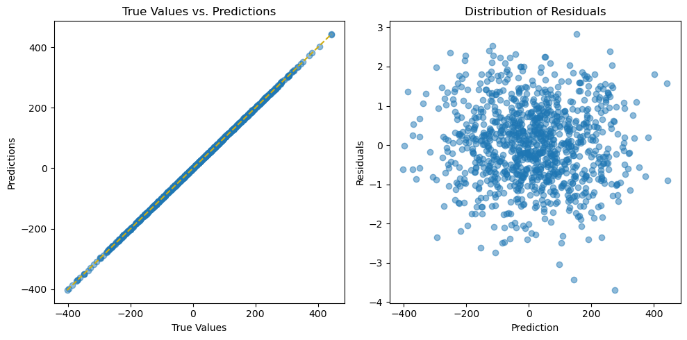
Mean Squared Error: 0.9917846740502066
[12]:
arfsfs.make_fs_summary(pipeline)
/home/bsatom/Documents/arfs/src/arfs/feature_selection/summary.py:69: FutureWarning: Styler.applymap has been deprecated. Use Styler.map instead.
  .applymap(lambda x: "" if x == x else "background-color: #f57505")
[12]:
| predictor | scaler | selector | linear_regression | |
|---|---|---|---|---|
| 0 | pred_0 | nan | 0 | nan |
| 1 | pred_1 | nan | 1 | nan |
| 2 | pred_2 | nan | 0 | nan |
| 3 | pred_3 | nan | 0 | nan |
| 4 | pred_4 | nan | 1 | nan |
| 5 | pred_5 | nan | 0 | nan |
| 6 | pred_6 | nan | 1 | nan |
| 7 | pred_7 | nan | 1 | nan |
| 8 | pred_8 | nan | 0 | nan |
| 9 | pred_9 | nan | 1 | nan |
[13]:
pipeline.named_steps["selector"].get_feature_names_out()
[13]:
Index(['Intercept', 'pred_1', 'pred_4', 'pred_6', 'pred_7', 'pred_9'], dtype='object')
beyond the feature selection quality, we can even check if the model itself is good.
[14]:
import seaborn as sns

# Plot the predictions and residuals
plt.figure(figsize=(10, 5))

# Plot predictions
plt.subplot(1, 2, 1)
plt.scatter(y_test, y_pred, alpha=0.5)
plt.plot(
    [min(y_test), max(y_test)],
    [min(y_test), max(y_test)],
    color="#d1ae11",
    linestyle="--",
)
plt.xlabel("True Values")
plt.ylabel("Predictions")
plt.title("True Values vs. Predictions")

# Plot residuals
residuals = y_test - y_pred
plt.subplot(1, 2, 2)
plt.scatter(y=residuals, x=y_pred, alpha=0.5)
plt.ylabel("Residuals")
plt.xlabel("Prediction")
plt.title("Distribution of Residuals")

plt.tight_layout()
plt.show();
Poisson toy example#
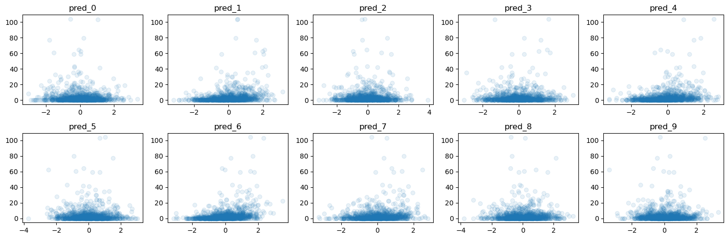
The loss can be one of the typical GLM losses: “gaussian”, “poisson”, “gamma”, “negativebinomial”, “binomial”, “tweedie”.
[15]:
# Generate synthetic data with Poisson-distributed target variable
bias = 1
X, y, true_coef = make_regression(
    n_samples=2_000,
    n_features=10,
    n_informative=5,
    noise=1,
    random_state=8,
    bias=bias,
    coef=True,
)
y = (y - y.mean()) / y.std()
y = np.exp(y)  # Transform to positive values for Poisson distribution
y = np.random.poisson(y)  # Add Poisson noise to the target variable
# dummy sample weight (e.g. exposure), smallest being 30 days
w = np.random.uniform(30 / 365, 1, size=len(y))
# make the count a Poisson rate (frequency)
y = y / w

X = pd.DataFrame(X)
X.columns = [f"pred_{i}" for i in range(X.shape[1])]

# Split the data into training and testing sets
X_train, X_test, y_train, y_test, w_train, w_test = train_test_split(
    X, y, w, test_size=0.5, random_state=42
)

print(f"The true coefficient of the linear data generating process are:\n {true_coef}")

f = plot_y_vs_X(X_train, y_train, ncols=5, figsize=(15, 5))
The true coefficient of the linear data generating process are:
 [ 0.         77.90364383  0.          0.         63.70230035  0.
 95.59499715 43.86990345  0.          4.11861919]
[16]:
y
[16]:
array([0.        , 2.34937393, 4.39264421, ..., 1.51556199, 5.72062399,
       0.        ])
[17]:
# Create a pipeline with LassoFeatureSelection and LinearRegression
pipeline = Pipeline(
    [
        ("scaler", StandardScaler()),
        (
            "selector",
            LassoFeatureSelection(
                n_iterations=10, score="bic", family="poisson", fit_intercept=True
            ),
        ),
        ("glm", PoissonRegressor()),
    ]
)

# Fit the pipeline to the training data
pipeline.fit(
    X_train, y_train, selector__sample_weight=w_train, glm__sample_weight=w_train
)
/home/bsatom/Documents/arfs_test_nbs/arfsuv/lib/python3.12/site-packages/sklearn/utils/deprecation.py:151: FutureWarning: 'force_all_finite' was renamed to 'ensure_all_finite' in 1.6 and will be removed in 1.8.
  warnings.warn(
[17]:
Pipeline(steps=[('scaler', StandardScaler()),
                ('selector', LassoFeatureSelection(family='poisson')),
                ('glm', PoissonRegressor())])
In a Jupyter environment, please rerun this cell to show the HTML representation or trust the notebook. On GitHub, the HTML representation is unable to render, please try loading this page with nbviewer.org.
Pipeline(steps=[('scaler', StandardScaler()),
                ('selector', LassoFeatureSelection(family='poisson')),
('glm', PoissonRegressor())])StandardScaler()
LassoFeatureSelection(family='poisson')
PoissonRegressor()
[18]:
import matplotlib.pyplot as plt
import seaborn as sns
from mpl_toolkits.axes_grid1.inset_locator import inset_axes

# Make predictions on the test set
y_pred = pipeline.predict(X_test)

# Calculate the residuals
residuals = y_test - y_pred

# Plot the predictions and residuals
fig, axs = plt.subplots(1, 2, figsize=(10, 5))

# Plot predictions
axs[0].scatter(y_test, y_pred, alpha=0.05)
axs[0].plot(
    [min(y_test), max(y_test)],
    [min(y_test), max(y_test)],
    color="#d1ae11",
    linestyle="--",
)
axs[0].set_xlabel("True Values")
axs[0].set_ylabel("Predictions")
axs[0].set_title("True Values vs. Predictions")


# Plot residuals
axs[1] = sns.histplot(residuals, kde=True, ax=axs[1])
axs[1].set_xlabel("Residuals")
axs[1].set_ylabel("Frequency")
axs[1].set_title("Distribution of Residuals")

plt.show();
[19]:
true_coef = pd.Series(true_coef)
true_coef.index = X.columns
true_coef = pd.Series({**{"intercept": bias}, **true_coef})
true_coef
[19]:
intercept     1.000000
pred_0        0.000000
pred_1       77.903644
pred_2        0.000000
pred_3        0.000000
pred_4       63.702300
pred_5        0.000000
pred_6       95.594997
pred_7       43.869903
pred_8        0.000000
pred_9        4.118619
dtype: float64
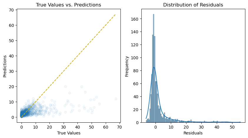
the selected predictors are
[20]:
pipeline.named_steps["selector"].get_feature_names_out()
[20]:
Index(['Intercept', 'pred_1', 'pred_4', 'pred_6', 'pred_7'], dtype='object')
[21]:
arfsfs.make_fs_summary(pipeline)
/home/bsatom/Documents/arfs/src/arfs/feature_selection/summary.py:69: FutureWarning: Styler.applymap has been deprecated. Use Styler.map instead.
  .applymap(lambda x: "" if x == x else "background-color: #f57505")
[21]:
| predictor | scaler | selector | glm | |
|---|---|---|---|---|
| 0 | pred_0 | nan | 0 | nan |
| 1 | pred_1 | nan | 1 | nan |
| 2 | pred_2 | nan | 0 | nan |
| 3 | pred_3 | nan | 0 | nan |
| 4 | pred_4 | nan | 1 | nan |
| 5 | pred_5 | nan | 0 | nan |
| 6 | pred_6 | nan | 1 | nan |
| 7 | pred_7 | nan | 1 | nan |
| 8 | pred_8 | nan | 0 | nan |
| 9 | pred_9 | nan | 0 | nan |
[22]:
pipeline.named_steps["selector"].best_estimator_.summary()
[22]:
| Dep. Variable: | y | No. Observations: | 1000 |
|---|---|---|---|
| Model: | GLM | Df Residuals: | 995 |
| Model Family: | Poisson | Df Model: | 5 |
| Link Function: | Log | Scale: | 1.0000 |
| Method: | elastic_net | Log-Likelihood: | -1295.4 |
| Date: | Wed, 02 Apr 2025 | Deviance: | 1561.5 |
| Time: | 16:13:02 | Pearson chi2: | 2.28e+03 |
| No. Iterations: | 24 | Pseudo R-squ. (CS): | 0.7581 |
| Covariance Type: | nonrobust |
| coef | std err | z | P>|z| | [0.025 | 0.975] | |
|---|---|---|---|---|---|---|
| Intercept | 0.6199 | 0.035 | 17.503 | 0.000 | 0.550 | 0.689 |
| pred_0 | 0 | 0 | nan | nan | 0 | 0 |
| pred_1 | 0.5340 | 0.026 | 20.859 | 0.000 | 0.484 | 0.584 |
| pred_2 | 0 | 0 | nan | nan | 0 | 0 |
| pred_3 | 0 | 0 | nan | nan | 0 | 0 |
| pred_4 | 0.4129 | 0.026 | 16.176 | 0.000 | 0.363 | 0.463 |
| pred_5 | 0 | 0 | nan | nan | 0 | 0 |
| pred_6 | 0.6096 | 0.026 | 23.814 | 0.000 | 0.559 | 0.660 |
| pred_7 | 0.3059 | 0.026 | 11.553 | 0.000 | 0.254 | 0.358 |
| pred_8 | 0 | 0 | nan | nan | 0 | 0 |
| pred_9 | 0 | 0 | nan | nan | 0 | 0 |
Categorical variable, missing values and miss-specified distribution#
When working with the PatsyTransformer, it’s essential to handle missing values in a specific way for categorical variables. To do this, we convert missing values into a string representation, as the native support of NaN in numpy is not yet fully implemented for general arrays.
Keep in mind that the dummy dataset we are using in this context does not necessarily correspond to any specific distribution assumption, such as the exponential family. However, for the purpose of feature selection, this might not pose a significant obstacle. The feature selection process can still be effective in identifying relevant predictors, even when the data does not precisely follow a specific distribution pattern.
Classical approach#
Unfortunatly, Patsy is not yet pickable, I’ll present to equivalent approaches, one pickable approach and another using the Patsy transformer.
[23]:
from arfs.utils import _make_corr_dataset_regression

X, y, w = _make_corr_dataset_regression(size=2_000)
# a dummy categorical variable with as many levels as rows
# and with zero variance
X = X.drop(columns=["var10", "var11"])
[24]:
# select all cols considered as categorical by numpy's standard'
from sklearn.impute import SimpleImputer
from sklearn.compose import ColumnTransformer
from sklearn.compose import make_column_selector as columns_selector
from sklearn.preprocessing import StandardScaler, OneHotEncoder

cat_features = columns_selector(dtype_include=["category", "object", "boolean"])
num_features = columns_selector(dtype_include=np.number)

numeric_transformer = Pipeline(
    steps=[
        ("imputer", SimpleImputer(missing_values=np.nan, strategy="median")),
        ("scaler", StandardScaler()),
    ]
)

categorical_transformer = Pipeline(
    steps=[
        (
            "imputer",
            SimpleImputer(
                missing_values=np.nan, strategy="constant", fill_value="Missing_Value"
            ),
        ),
        ("encoder", OneHotEncoder(handle_unknown="ignore", sparse_output=False)),
    ]
)


preprocessor = ColumnTransformer(
    transformers=[
        ("num", numeric_transformer, num_features),
        ("cat", categorical_transformer, cat_features),
    ],
    remainder="passthrough",
    verbose_feature_names_out=False,
).set_output(transform="pandas")


# Create the pipeline
pipeline = Pipeline(
    [
        ("preprocess", preprocessor),
        (
            "selector",
            LassoFeatureSelection(
                n_iterations=10, score="bic", family="gaussian", fit_intercept=True
            ),
        ),
    ]
)

# Fit the model
pipeline.fit(X, y)  # , selector__sample_weight=w)
/home/bsatom/Documents/arfs_test_nbs/arfsuv/lib/python3.12/site-packages/sklearn/utils/deprecation.py:151: FutureWarning: 'force_all_finite' was renamed to 'ensure_all_finite' in 1.6 and will be removed in 1.8.
  warnings.warn(
/home/bsatom/Documents/arfs_test_nbs/arfsuv/lib/python3.12/site-packages/statsmodels/genmod/generalized_linear_model.py:1464: UserWarning: Elastic net fitting did not converge
  warnings.warn("Elastic net fitting did not converge")
/home/bsatom/Documents/arfs_test_nbs/arfsuv/lib/python3.12/site-packages/statsmodels/genmod/generalized_linear_model.py:1464: UserWarning: Elastic net fitting did not converge
  warnings.warn("Elastic net fitting did not converge")
/home/bsatom/Documents/arfs_test_nbs/arfsuv/lib/python3.12/site-packages/statsmodels/genmod/generalized_linear_model.py:1464: UserWarning: Elastic net fitting did not converge
  warnings.warn("Elastic net fitting did not converge")
/home/bsatom/Documents/arfs_test_nbs/arfsuv/lib/python3.12/site-packages/statsmodels/genmod/generalized_linear_model.py:1464: UserWarning: Elastic net fitting did not converge
  warnings.warn("Elastic net fitting did not converge")
[24]:
Pipeline(steps=[('preprocess',
                 ColumnTransformer(remainder='passthrough',
                                   transformers=[('num',
                                                  Pipeline(steps=[('imputer',
                                                                   SimpleImputer(strategy='median')),
                                                                  ('scaler',
                                                                   StandardScaler())]),
                                                  <sklearn.compose._column_transformer.make_column_selector object at 0x7c305ab06540>),
                                                 ('cat',
                                                  Pipeline(steps=[('imputer',
                                                                   SimpleImputer(fill_value='Missing_Value',
                                                                                 strategy='constant')),
                                                                  ('encoder',
                                                                   OneHotEncoder(handle_unknown='ignore',
                                                                                 sparse_output=False))]),
                                                  <sklearn.compose._column_transformer.make_column_selector object at 0x7c30597e0c80>)],
                                   verbose_feature_names_out=False)),
                ('selector', LassoFeatureSelection())])
In a Jupyter environment, please rerun this cell to show the HTML representation or trust the notebook. On GitHub, the HTML representation is unable to render, please try loading this page with nbviewer.org.
Pipeline(steps=[('preprocess',
                 ColumnTransformer(remainder='passthrough',
                                   transformers=[('num',
                                                  Pipeline(steps=[('imputer',
                                                                   SimpleImputer(strategy='median')),
                                                                  ('scaler',
                                                                   StandardScaler())]),
                                                  <sklearn.compose._column_transformer.make_column_selector object at 0x7c305ab06540>),
                                                 ('cat',
                                                  Pipeline(steps=[('imputer',
                                                                   SimpleImputer(fill_value='Missing_Value',
                                                                                 strategy='constant')),
                                                                  ('encoder',
                                                                   OneHotEncoder(handle_unknown='ignore',
                                                                                 sparse_output=False))]),
                                                  <sklearn.compose._column_transformer.make_column_selector object at 0x7c30597e0c80>)],
                                   verbose_feature_names_out=False)),
('selector', LassoFeatureSelection())])ColumnTransformer(remainder='passthrough',
transformers=[('num',
Pipeline(steps=[('imputer',
SimpleImputer(strategy='median')),
('scaler', StandardScaler())]),
<sklearn.compose._column_transformer.make_column_selector object at 0x7c305ab06540>),
('cat',
Pipeline(steps=[('imputer',
SimpleImputer(fill_value='Missing_Value',
strategy='constant')),
('encoder',
OneHotEncoder(handle_unknown='ignore',
sparse_output=False))]),
<sklearn.compose._column_transformer.make_column_selector object at 0x7c30597e0c80>)],
verbose_feature_names_out=False)<sklearn.compose._column_transformer.make_column_selector object at 0x7c305ab06540>
SimpleImputer(strategy='median')
StandardScaler()
<sklearn.compose._column_transformer.make_column_selector object at 0x7c30597e0c80>
SimpleImputer(fill_value='Missing_Value', strategy='constant')
OneHotEncoder(handle_unknown='ignore', sparse_output=False)
[]
passthrough
LassoFeatureSelection()
[25]:
arfsfs.make_fs_summary(pipeline)
/home/bsatom/Documents/arfs/src/arfs/feature_selection/summary.py:69: FutureWarning: Styler.applymap has been deprecated. Use Styler.map instead.
  .applymap(lambda x: "" if x == x else "background-color: #f57505")
[25]:
| predictor | preprocess | selector | |
|---|---|---|---|
| 0 | var0 | nan | 1 |
| 1 | var1 | nan | 1 |
| 2 | var2 | nan | 1 |
| 3 | var3 | nan | 1 |
| 4 | var4 | nan | 1 |
| 5 | var5 | nan | 1 |
| 6 | var6 | nan | 0 |
| 7 | var7 | nan | 0 |
| 8 | var8 | nan | 0 |
| 9 | var9 | nan | 0 |
| 10 | var12 | nan | 0 |
| 11 | nice_guys | nan | nan |
[26]:
pipeline.named_steps["selector"].get_feature_names_out()
[26]:
Index(['Intercept', 'var0', 'var1', 'var2', 'var3', 'var4', 'var5'], dtype='object')
[27]:
pipeline.named_steps["selector"].feature_names_in_
[27]:
Index(['Intercept', 'var0', 'var1', 'var2', 'var3', 'var4', 'var5', 'var6',
       'var7', 'var8', 'var9', 'var12', 'nice_guys_Alien', 'nice_guys_Bane',
       'nice_guys_Bejita', 'nice_guys_Bender', 'nice_guys_Bias',
       'nice_guys_Blackbeard', 'nice_guys_Cartman', 'nice_guys_Cell',
       'nice_guys_Coldplay', 'nice_guys_Creationist', 'nice_guys_Dracula',
       'nice_guys_Drago', 'nice_guys_Excel', 'nice_guys_Fry',
       'nice_guys_Garry', 'nice_guys_Geoffrey', 'nice_guys_Goldfinder',
       'nice_guys_Gruber', 'nice_guys_Human', 'nice_guys_Imaginedragons',
       'nice_guys_KeyserSoze', 'nice_guys_Klaue', 'nice_guys_Krueger',
       'nice_guys_Lecter', 'nice_guys_Luthor', 'nice_guys_MarkZ',
       'nice_guys_Morty', 'nice_guys_Platist', 'nice_guys_Rick',
       'nice_guys_SAS', 'nice_guys_Scrum', 'nice_guys_Terminator',
       'nice_guys_Thanos', 'nice_guys_Tinkywinky', 'nice_guys_Vador',
       'nice_guys_Variance'],
      dtype='object')
Using the Patsy transformer
[28]:
cat_features = columns_selector(dtype_include=["category", "object", "boolean"])
num_features = columns_selector(dtype_include=np.number)

numeric_transformer = Pipeline(
    steps=[
        ("imputer", SimpleImputer(missing_values=np.nan, strategy="median")),
        ("scaler", StandardScaler()),
    ]
)

# either drop the NA or impute them
imputer = ColumnTransformer(
    transformers=[
        (
            "cat",
            SimpleImputer(
                missing_values=np.nan, strategy="constant", fill_value="Missing_Value"
            ),
            cat_features,
        ),
        ("num", numeric_transformer, num_features),
    ],
    remainder="passthrough",
    verbose_feature_names_out=False,
).set_output(transform="pandas")

# Create the pipeline
pipeline = Pipeline(
    [
        ("imputer", imputer),
        ("preprocess", PatsyTransformer()),
        (
            "selector",
            LassoFeatureSelection(
                n_iterations=10, score="bic", family="gaussian", fit_intercept=True
            ),
        ),
    ]
)

# Fit the model
pipeline.fit(X, y)  # , selector__sample_weight=w)
/home/bsatom/Documents/arfs_test_nbs/arfsuv/lib/python3.12/site-packages/sklearn/utils/deprecation.py:151: FutureWarning: 'force_all_finite' was renamed to 'ensure_all_finite' in 1.6 and will be removed in 1.8.
  warnings.warn(
/home/bsatom/Documents/arfs_test_nbs/arfsuv/lib/python3.12/site-packages/statsmodels/genmod/generalized_linear_model.py:1464: UserWarning: Elastic net fitting did not converge
  warnings.warn("Elastic net fitting did not converge")
/home/bsatom/Documents/arfs_test_nbs/arfsuv/lib/python3.12/site-packages/statsmodels/genmod/generalized_linear_model.py:1464: UserWarning: Elastic net fitting did not converge
  warnings.warn("Elastic net fitting did not converge")
[28]:
Pipeline(steps=[('imputer',
                 ColumnTransformer(remainder='passthrough',
                                   transformers=[('cat',
                                                  SimpleImputer(fill_value='Missing_Value',
                                                                strategy='constant'),
                                                  <sklearn.compose._column_transformer.make_column_selector object at 0x7c3058c2ffe0>),
                                                 ('num',
                                                  Pipeline(steps=[('imputer',
                                                                   SimpleImputer(strategy='median')),
                                                                  ('scaler',
                                                                   StandardScaler())]),
                                                  <sklearn.compose._column_transformer.make_column_selector object at 0x7c3058c2c830>)],
                                   verbose_feature_names_out=False)),
                ('preprocess',
                 PatsyTransformer(formula='nice_guys + var0 + var1 + var12 + '
                                          'var2 + var3 + var4 + var5 + var6 + '
                                          'var7 + var8 + var9')),
                ('selector', LassoFeatureSelection())])
In a Jupyter environment, please rerun this cell to show the HTML representation or trust the notebook. On GitHub, the HTML representation is unable to render, please try loading this page with nbviewer.org.
Pipeline(steps=[('imputer',
                 ColumnTransformer(remainder='passthrough',
                                   transformers=[('cat',
                                                  SimpleImputer(fill_value='Missing_Value',
                                                                strategy='constant'),
                                                  <sklearn.compose._column_transformer.make_column_selector object at 0x7c3058c2ffe0>),
                                                 ('num',
                                                  Pipeline(steps=[('imputer',
                                                                   SimpleImputer(strategy='median')),
                                                                  ('scaler',
                                                                   StandardScaler())]),
                                                  <sklearn.compose._column_transformer.make_column_selector object at 0x7c3058c2c830>)],
                                   verbose_feature_names_out=False)),
                ('preprocess',
                 PatsyTransformer(formula='nice_guys + var0 + var1 + var12 + '
                                          'var2 + var3 + var4 + var5 + var6 + '
                                          'var7 + var8 + var9')),
('selector', LassoFeatureSelection())])ColumnTransformer(remainder='passthrough',
transformers=[('cat',
SimpleImputer(fill_value='Missing_Value',
strategy='constant'),
<sklearn.compose._column_transformer.make_column_selector object at 0x7c3058c2ffe0>),
('num',
Pipeline(steps=[('imputer',
SimpleImputer(strategy='median')),
('scaler', StandardScaler())]),
<sklearn.compose._column_transformer.make_column_selector object at 0x7c3058c2c830>)],
verbose_feature_names_out=False)<sklearn.compose._column_transformer.make_column_selector object at 0x7c3058c2ffe0>
SimpleImputer(fill_value='Missing_Value', strategy='constant')
<sklearn.compose._column_transformer.make_column_selector object at 0x7c3058c2c830>
SimpleImputer(strategy='median')
StandardScaler()
[]
passthrough
PatsyTransformer(formula='nice_guys + var0 + var1 + var12 + var2 + var3 + var4 '
'+ var5 + var6 + var7 + var8 + var9')LassoFeatureSelection()
[29]:
f = plot_y_vs_X(X, y, ncols=7, figsize=(16, 4))
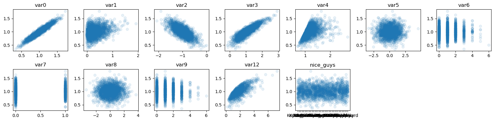
The genuine predictors are : var0, var1, var2, var3, var4 and var12
[30]:
X.head()
[30]:
| var0 | var1 | var2 | var3 | var4 | var5 | var6 | var7 | var8 | var9 | var12 | nice_guys | |
|---|---|---|---|---|---|---|---|---|---|---|---|---|
| 0 | 1.091810 | 0.489242 | -1.235042 | 1.443517 | 1.084685 | 0.716430 | 2 | 0 | 0.532132 | 1 | 2.212539 | Krueger |
| 1 | 0.976880 | 0.235321 | -1.033447 | 0.569663 | 1.017232 | 1.155733 | 1 | 1 | 0.147567 | 1 | 0.919993 | KeyserSoze |
| 2 | 1.161955 | 0.422190 | -1.249014 | 1.210296 | 1.218725 | -3.307900 | 1 | 0 | -0.295357 | 2 | 1.506035 | Klaue |
| 3 | 1.335830 | 0.300262 | -1.282522 | 1.693665 | 1.332802 | -0.151363 | 1 | 0 | -0.740745 | 3 | NaN | Bane |
| 4 | 0.974240 | 0.107206 | -0.713734 | 0.911713 | 1.107156 | -2.875773 | 2 | 0 | 0.112322 | 1 | 1.971962 | Krueger |
[31]:
arfsfs.make_fs_summary(pipeline)
/home/bsatom/Documents/arfs/src/arfs/feature_selection/summary.py:69: FutureWarning: Styler.applymap has been deprecated. Use Styler.map instead.
  .applymap(lambda x: "" if x == x else "background-color: #f57505")
[31]:
| predictor | imputer | preprocess | selector | |
|---|---|---|---|---|
| 0 | var0 | nan | nan | 1 |
| 1 | var1 | nan | nan | 1 |
| 2 | var2 | nan | nan | 1 |
| 3 | var3 | nan | nan | 1 |
| 4 | var4 | nan | nan | 1 |
| 5 | var5 | nan | nan | 1 |
| 6 | var6 | nan | nan | 0 |
| 7 | var7 | nan | nan | 0 |
| 8 | var8 | nan | nan | 0 |
| 9 | var9 | nan | nan | 0 |
| 10 | var12 | nan | nan | 1 |
| 11 | nice_guys | nan | nan | nan |
[32]:
pipeline.named_steps["selector"].get_feature_names_out()
[32]:
Index(['Intercept', 'var0', 'var1', 'var12', 'var2', 'var3', 'var4', 'var5'], dtype='object')
[33]:
pipeline.named_steps["selector"].support_
[33]:
array([ True, False, False, False, False, False, False, False, False,
       False, False, False, False, False, False, False, False, False,
       False, False, False, False, False, False, False, False, False,
       False, False, False, False, False, False, False, False, False,
        True,  True,  True,  True,  True,  True,  True, False, False,
       False, False])
[34]:
X_trans = pipeline.transform(X)
X_trans.head()
[34]:
| Intercept | var0 | var1 | var12 | var2 | var3 | var4 | var5 | |
|---|---|---|---|---|---|---|---|---|
| 0 | 1.0 | 0.410244 | 0.579520 | 0.515223 | -0.785263 | 0.844345 | -0.518385 | 0.683297 |
| 1 | 1.0 | -0.148030 | -0.373188 | -1.496868 | -0.068675 | -1.102092 | -0.803974 | 1.120786 |
| 2 | 1.0 | 0.750973 | 0.327939 | -0.584584 | -0.834928 | 0.324865 | 0.049133 | -3.324418 |
| 3 | 1.0 | 1.595568 | -0.129529 | -0.083170 | -0.954037 | 1.401527 | 0.532125 | -0.180913 |
| 4 | 1.0 | -0.160855 | -0.853871 | 0.140719 | 1.067778 | -0.340203 | -0.423244 | -2.894075 |
[35]:
pipeline.named_steps["selector"].feature_names_in_
[35]:
Index(['Intercept', 'nice_guys[T.Bane]', 'nice_guys[T.Bejita]',
       'nice_guys[T.Bender]', 'nice_guys[T.Bias]', 'nice_guys[T.Blackbeard]',
       'nice_guys[T.Cartman]', 'nice_guys[T.Cell]', 'nice_guys[T.Coldplay]',
       'nice_guys[T.Creationist]', 'nice_guys[T.Dracula]',
       'nice_guys[T.Drago]', 'nice_guys[T.Excel]', 'nice_guys[T.Fry]',
       'nice_guys[T.Garry]', 'nice_guys[T.Geoffrey]',
       'nice_guys[T.Goldfinder]', 'nice_guys[T.Gruber]', 'nice_guys[T.Human]',
       'nice_guys[T.Imaginedragons]', 'nice_guys[T.KeyserSoze]',
       'nice_guys[T.Klaue]', 'nice_guys[T.Krueger]', 'nice_guys[T.Lecter]',
       'nice_guys[T.Luthor]', 'nice_guys[T.MarkZ]', 'nice_guys[T.Morty]',
       'nice_guys[T.Platist]', 'nice_guys[T.Rick]', 'nice_guys[T.SAS]',
       'nice_guys[T.Scrum]', 'nice_guys[T.Terminator]', 'nice_guys[T.Thanos]',
       'nice_guys[T.Tinkywinky]', 'nice_guys[T.Vador]',
       'nice_guys[T.Variance]', 'var0', 'var1', 'var12', 'var2', 'var3',
       'var4', 'var5', 'var6', 'var7', 'var8', 'var9'],
      dtype='object')
[36]:
pipeline.named_steps["selector"].best_estimator_.summary()
[36]:
| Dep. Variable: | y | No. Observations: | 2000 |
|---|---|---|---|
| Model: | GLM | Df Residuals: | 1992 |
| Model Family: | Gaussian | Df Model: | 8 |
| Link Function: | Identity | Scale: | 0.0021507 |
| Method: | elastic_net | Log-Likelihood: | 3308.1 |
| Date: | Wed, 02 Apr 2025 | Deviance: | 4.2841 |
| Time: | 16:13:19 | Pearson chi2: | 4.28 |
| No. Iterations: | 49 | Pseudo R-squ. (CS): | 1.000 |
| Covariance Type: | nonrobust |
| coef | std err | z | P>|z| | [0.025 | 0.975] | |
|---|---|---|---|---|---|---|
| Intercept | 1.0090 | 0.001 | 973.031 | 0.000 | 1.007 | 1.011 |
| nice_guys[T.Bane] | 0 | 0 | nan | nan | 0 | 0 |
| nice_guys[T.Bejita] | 0 | 0 | nan | nan | 0 | 0 |
| nice_guys[T.Bender] | 0 | 0 | nan | nan | 0 | 0 |
| nice_guys[T.Bias] | 0 | 0 | nan | nan | 0 | 0 |
| nice_guys[T.Blackbeard] | 0 | 0 | nan | nan | 0 | 0 |
| nice_guys[T.Cartman] | 0 | 0 | nan | nan | 0 | 0 |
| nice_guys[T.Cell] | 0 | 0 | nan | nan | 0 | 0 |
| nice_guys[T.Coldplay] | 0 | 0 | nan | nan | 0 | 0 |
| nice_guys[T.Creationist] | 0 | 0 | nan | nan | 0 | 0 |
| nice_guys[T.Dracula] | 0 | 0 | nan | nan | 0 | 0 |
| nice_guys[T.Drago] | 0 | 0 | nan | nan | 0 | 0 |
| nice_guys[T.Excel] | 0 | 0 | nan | nan | 0 | 0 |
| nice_guys[T.Fry] | 0 | 0 | nan | nan | 0 | 0 |
| nice_guys[T.Garry] | 0 | 0 | nan | nan | 0 | 0 |
| nice_guys[T.Geoffrey] | 0 | 0 | nan | nan | 0 | 0 |
| nice_guys[T.Goldfinder] | 0 | 0 | nan | nan | 0 | 0 |
| nice_guys[T.Gruber] | 0 | 0 | nan | nan | 0 | 0 |
| nice_guys[T.Human] | 0 | 0 | nan | nan | 0 | 0 |
| nice_guys[T.Imaginedragons] | 0 | 0 | nan | nan | 0 | 0 |
| nice_guys[T.KeyserSoze] | 0 | 0 | nan | nan | 0 | 0 |
| nice_guys[T.Klaue] | 0 | 0 | nan | nan | 0 | 0 |
| nice_guys[T.Krueger] | 0 | 0 | nan | nan | 0 | 0 |
| nice_guys[T.Lecter] | 0 | 0 | nan | nan | 0 | 0 |
| nice_guys[T.Luthor] | 0 | 0 | nan | nan | 0 | 0 |
| nice_guys[T.MarkZ] | 0 | 0 | nan | nan | 0 | 0 |
| nice_guys[T.Morty] | 0 | 0 | nan | nan | 0 | 0 |
| nice_guys[T.Platist] | 0 | 0 | nan | nan | 0 | 0 |
| nice_guys[T.Rick] | 0 | 0 | nan | nan | 0 | 0 |
| nice_guys[T.SAS] | 0 | 0 | nan | nan | 0 | 0 |
| nice_guys[T.Scrum] | 0 | 0 | nan | nan | 0 | 0 |
| nice_guys[T.Terminator] | 0 | 0 | nan | nan | 0 | 0 |
| nice_guys[T.Thanos] | 0 | 0 | nan | nan | 0 | 0 |
| nice_guys[T.Tinkywinky] | 0 | 0 | nan | nan | 0 | 0 |
| nice_guys[T.Vador] | 0 | 0 | nan | nan | 0 | 0 |
| nice_guys[T.Variance] | 0 | 0 | nan | nan | 0 | 0 |
| var0 | 0.1400 | 0.002 | 63.092 | 0.000 | 0.136 | 0.144 |
| var1 | 0.0022 | 0.001 | 2.065 | 0.039 | 0.000 | 0.004 |
| var12 | 0.0038 | 0.001 | 3.170 | 0.002 | 0.001 | 0.006 |
| var2 | -0.0152 | 0.001 | -10.635 | 0.000 | -0.018 | -0.012 |
| var3 | 0.0411 | 0.002 | 20.080 | 0.000 | 0.037 | 0.045 |
| var4 | 0.0053 | 0.001 | 4.606 | 0.000 | 0.003 | 0.008 |
| var5 | -0.0014 | 0.001 | -1.379 | 0.168 | -0.003 | 0.001 |
| var6 | 0 | 0 | nan | nan | 0 | 0 |
| var7 | 0 | 0 | nan | nan | 0 | 0 |
| var8 | 0 | 0 | nan | nan | 0 | 0 |
| var9 | 0 | 0 | nan | nan | 0 | 0 |
Advanced approach#
We can auto-bin the predictors and group levels. The non-informative predictors will not be binned and their value will be np.nan or np.Inf
[37]:
from arfs.preprocessing import TreeDiscretizer, IntervalToMidpoint
from arfs.feature_selection import UniqueValuesThreshold, MissingValueThreshold

cat_features = columns_selector(dtype_include=["category", "object", "boolean"])
num_features = columns_selector(dtype_include=np.number)

preprocessor = ColumnTransformer(
    transformers=[
        ("num", StandardScaler(), num_features),
        (
            "cat",
            OneHotEncoder(handle_unknown="ignore", sparse_output=False),
            cat_features,
        ),
    ],
    remainder="passthrough",
    verbose_feature_names_out=False,
).set_output(transform="pandas")


# Create the pipeline
pipeline = Pipeline(
    [
        (
            "disctretizer",
            TreeDiscretizer(
                bin_features="all", n_bins=10, boost_params={"min_split_gain": 0.05}
            ),
        ),
        ("midpointer", IntervalToMidpoint()),
        ("zero_variance", UniqueValuesThreshold()),
        # the treediscretization might introduce NaN for pure noise columns
        ("missing", MissingValueThreshold(0.05)),
        ("preprocess", preprocessor),
        (
            "selector",
            LassoFeatureSelection(
                n_iterations=10, score="bic", family="gaussian", fit_intercept=True
            ),
        ),
    ]
)

pipeline.fit(X, y)
Data split: Train=1600 samples, Validation=400 samples.
No 'metric' provided, using objective 'rmse' as metric.
Training up to 1 boosting rounds.
/home/bsatom/Documents/arfs/src/arfs/gbm.py:339: UserWarning: Model was trained with feature names, but input X for prediction is not a DataFrame. Converting.
  warnings.warn("Model was trained with feature names, but input X for prediction is not a DataFrame. Converting.")
/home/bsatom/Documents/arfs/src/arfs/gbm.py:339: UserWarning: Model was trained with feature names, but input X for prediction is not a DataFrame. Converting.
  warnings.warn("Model was trained with feature names, but input X for prediction is not a DataFrame. Converting.")
/home/bsatom/Documents/arfs/src/arfs/gbm.py:339: UserWarning: Model was trained with feature names, but input X for prediction is not a DataFrame. Converting.
  warnings.warn("Model was trained with feature names, but input X for prediction is not a DataFrame. Converting.")
Data split: Train=1600 samples, Validation=400 samples.
No 'metric' provided, using objective 'rmse' as metric.
Training up to 1 boosting rounds.
Data split: Train=1600 samples, Validation=400 samples.
No 'metric' provided, using objective 'rmse' as metric.
Training up to 1 boosting rounds.
/home/bsatom/Documents/arfs/src/arfs/gbm.py:339: UserWarning: Model was trained with feature names, but input X for prediction is not a DataFrame. Converting.
  warnings.warn("Model was trained with feature names, but input X for prediction is not a DataFrame. Converting.")
/home/bsatom/Documents/arfs/src/arfs/gbm.py:339: UserWarning: Model was trained with feature names, but input X for prediction is not a DataFrame. Converting.
  warnings.warn("Model was trained with feature names, but input X for prediction is not a DataFrame. Converting.")
/home/bsatom/Documents/arfs/src/arfs/gbm.py:339: UserWarning: Model was trained with feature names, but input X for prediction is not a DataFrame. Converting.
  warnings.warn("Model was trained with feature names, but input X for prediction is not a DataFrame. Converting.")
Data split: Train=1600 samples, Validation=400 samples.
No 'metric' provided, using objective 'rmse' as metric.
Training up to 1 boosting rounds.
Data split: Train=1600 samples, Validation=400 samples.
No 'metric' provided, using objective 'rmse' as metric.
Training up to 1 boosting rounds.
/home/bsatom/Documents/arfs/src/arfs/gbm.py:339: UserWarning: Model was trained with feature names, but input X for prediction is not a DataFrame. Converting.
  warnings.warn("Model was trained with feature names, but input X for prediction is not a DataFrame. Converting.")
/home/bsatom/Documents/arfs/src/arfs/gbm.py:339: UserWarning: Model was trained with feature names, but input X for prediction is not a DataFrame. Converting.
  warnings.warn("Model was trained with feature names, but input X for prediction is not a DataFrame. Converting.")
/home/bsatom/Documents/arfs/src/arfs/gbm.py:339: UserWarning: Model was trained with feature names, but input X for prediction is not a DataFrame. Converting.
  warnings.warn("Model was trained with feature names, but input X for prediction is not a DataFrame. Converting.")
/home/bsatom/Documents/arfs/src/arfs/gbm.py:339: UserWarning: Model was trained with feature names, but input X for prediction is not a DataFrame. Converting.
  warnings.warn("Model was trained with feature names, but input X for prediction is not a DataFrame. Converting.")
Data split: Train=1600 samples, Validation=400 samples.
No 'metric' provided, using objective 'rmse' as metric.
Training up to 1 boosting rounds.
Data split: Train=1600 samples, Validation=400 samples.
No 'metric' provided, using objective 'rmse' as metric.
Training up to 1 boosting rounds.
/home/bsatom/Documents/arfs/src/arfs/gbm.py:339: UserWarning: Model was trained with feature names, but input X for prediction is not a DataFrame. Converting.
  warnings.warn("Model was trained with feature names, but input X for prediction is not a DataFrame. Converting.")
/home/bsatom/Documents/arfs/src/arfs/gbm.py:339: UserWarning: Model was trained with feature names, but input X for prediction is not a DataFrame. Converting.
  warnings.warn("Model was trained with feature names, but input X for prediction is not a DataFrame. Converting.")
/home/bsatom/Documents/arfs/src/arfs/gbm.py:339: UserWarning: Model was trained with feature names, but input X for prediction is not a DataFrame. Converting.
  warnings.warn("Model was trained with feature names, but input X for prediction is not a DataFrame. Converting.")
/home/bsatom/Documents/arfs/src/arfs/gbm.py:339: UserWarning: Model was trained with feature names, but input X for prediction is not a DataFrame. Converting.
  warnings.warn("Model was trained with feature names, but input X for prediction is not a DataFrame. Converting.")
Data split: Train=1600 samples, Validation=400 samples.
No 'metric' provided, using objective 'rmse' as metric.
Training up to 1 boosting rounds.
Data split: Train=1600 samples, Validation=400 samples.
No 'metric' provided, using objective 'rmse' as metric.
Training up to 1 boosting rounds.
/home/bsatom/Documents/arfs/src/arfs/gbm.py:339: UserWarning: Model was trained with feature names, but input X for prediction is not a DataFrame. Converting.
  warnings.warn("Model was trained with feature names, but input X for prediction is not a DataFrame. Converting.")
/home/bsatom/Documents/arfs/src/arfs/gbm.py:339: UserWarning: Model was trained with feature names, but input X for prediction is not a DataFrame. Converting.
  warnings.warn("Model was trained with feature names, but input X for prediction is not a DataFrame. Converting.")
/home/bsatom/Documents/arfs/src/arfs/gbm.py:339: UserWarning: Model was trained with feature names, but input X for prediction is not a DataFrame. Converting.
  warnings.warn("Model was trained with feature names, but input X for prediction is not a DataFrame. Converting.")
/home/bsatom/Documents/arfs/src/arfs/gbm.py:339: UserWarning: Model was trained with feature names, but input X for prediction is not a DataFrame. Converting.
  warnings.warn("Model was trained with feature names, but input X for prediction is not a DataFrame. Converting.")
Data split: Train=1600 samples, Validation=400 samples.
No 'metric' provided, using objective 'rmse' as metric.
Training up to 1 boosting rounds.
Data split: Train=1600 samples, Validation=400 samples.
No 'metric' provided, using objective 'rmse' as metric.
Training up to 1 boosting rounds.
/home/bsatom/Documents/arfs/src/arfs/gbm.py:339: UserWarning: Model was trained with feature names, but input X for prediction is not a DataFrame. Converting.
  warnings.warn("Model was trained with feature names, but input X for prediction is not a DataFrame. Converting.")
/home/bsatom/Documents/arfs/src/arfs/gbm.py:339: UserWarning: Model was trained with feature names, but input X for prediction is not a DataFrame. Converting.
  warnings.warn("Model was trained with feature names, but input X for prediction is not a DataFrame. Converting.")
/home/bsatom/Documents/arfs/src/arfs/gbm.py:339: UserWarning: Model was trained with feature names, but input X for prediction is not a DataFrame. Converting.
  warnings.warn("Model was trained with feature names, but input X for prediction is not a DataFrame. Converting.")
/home/bsatom/Documents/arfs/src/arfs/preprocessing.py:783: FutureWarning: Setting an item of incompatible dtype is deprecated and will raise in a future error of pandas. Value '[ 0.75   1.115 -0.51  ...  1.65  -0.51   0.615]' has dtype incompatible with interval[float64, right], please explicitly cast to a compatible dtype first.
  X.loc[:, c] = find_interval_midpoint(X[c])
/home/bsatom/Documents/arfs/src/arfs/preprocessing.py:783: FutureWarning: Setting an item of incompatible dtype is deprecated and will raise in a future error of pandas. Value '[-1.305 -1.04  -1.305 ... -0.635 -1.04  -1.04 ]' has dtype incompatible with interval[float64, right], please explicitly cast to a compatible dtype first.
  X.loc[:, c] = find_interval_midpoint(X[c])
/home/bsatom/Documents/arfs/src/arfs/preprocessing.py:783: FutureWarning: Setting an item of incompatible dtype is deprecated and will raise in a future error of pandas. Value '[2. 2. 2. ... 2. 2. 2.]' has dtype incompatible with interval[float64, right], please explicitly cast to a compatible dtype first.
  X.loc[:, c] = find_interval_midpoint(X[c])
/home/bsatom/Documents/arfs/src/arfs/preprocessing.py:783: FutureWarning: Setting an item of incompatible dtype is deprecated and will raise in a future error of pandas. Value '[inf inf inf ... inf inf inf]' has dtype incompatible with interval[float64, right], please explicitly cast to a compatible dtype first.
  X.loc[:, c] = find_interval_midpoint(X[c])
/home/bsatom/Documents/arfs/src/arfs/preprocessing.py:783: FutureWarning: Setting an item of incompatible dtype is deprecated and will raise in a future error of pandas. Value '[1.145 0.96  1.145 ... 0.845 0.96  0.845]' has dtype incompatible with interval[float64, right], please explicitly cast to a compatible dtype first.
  X.loc[:, c] = find_interval_midpoint(X[c])
/home/bsatom/Documents/arfs/src/arfs/preprocessing.py:783: FutureWarning: Setting an item of incompatible dtype is deprecated and will raise in a future error of pandas. Value '[1.375 0.58  1.145 ... 0.58  0.92  0.73 ]' has dtype incompatible with interval[float64, right], please explicitly cast to a compatible dtype first.
  X.loc[:, c] = find_interval_midpoint(X[c])
/home/bsatom/Documents/arfs/src/arfs/preprocessing.py:783: FutureWarning: Setting an item of incompatible dtype is deprecated and will raise in a future error of pandas. Value '[1.09  0.99  1.185 ... 0.99  1.04  1.185]' has dtype incompatible with interval[float64, right], please explicitly cast to a compatible dtype first.
  X.loc[:, c] = find_interval_midpoint(X[c])
/home/bsatom/Documents/arfs/src/arfs/preprocessing.py:783: FutureWarning: Setting an item of incompatible dtype is deprecated and will raise in a future error of pandas. Value '[ 0.585  0.285 -0.245 ... -0.55  -0.92   0.585]' has dtype incompatible with interval[float64, right], please explicitly cast to a compatible dtype first.
  X.loc[:, c] = find_interval_midpoint(X[c])
/home/bsatom/Documents/arfs/src/arfs/preprocessing.py:783: FutureWarning: Setting an item of incompatible dtype is deprecated and will raise in a future error of pandas. Value '[2.07  1.04  1.405 ... 1.405 1.04  1.775]' has dtype incompatible with interval[float64, right], please explicitly cast to a compatible dtype first.
  X.loc[:, c] = find_interval_midpoint(X[c])
/home/bsatom/Documents/arfs/src/arfs/preprocessing.py:783: FutureWarning: Setting an item of incompatible dtype is deprecated and will raise in a future error of pandas. Value '[0.54  0.27  0.37  ... 0.27  0.63  0.865]' has dtype incompatible with interval[float64, right], please explicitly cast to a compatible dtype first.
  X.loc[:, c] = find_interval_midpoint(X[c])
/home/bsatom/Documents/arfs/src/arfs/preprocessing.py:783: FutureWarning: Setting an item of incompatible dtype is deprecated and will raise in a future error of pandas. Value '[inf inf inf ... inf inf inf]' has dtype incompatible with interval[float64, right], please explicitly cast to a compatible dtype first.
  X.loc[:, c] = find_interval_midpoint(X[c])
/home/bsatom/Documents/arfs_test_nbs/arfsuv/lib/python3.12/site-packages/sklearn/utils/deprecation.py:151: FutureWarning: 'force_all_finite' was renamed to 'ensure_all_finite' in 1.6 and will be removed in 1.8.
  warnings.warn(
/home/bsatom/Documents/arfs_test_nbs/arfsuv/lib/python3.12/site-packages/statsmodels/genmod/generalized_linear_model.py:1464: UserWarning: Elastic net fitting did not converge
  warnings.warn("Elastic net fitting did not converge")
[37]:
Pipeline(steps=[('disctretizer',
                 TreeDiscretizer(bin_features=['var0', 'var1', 'var2', 'var3',
                                               'var4', 'var5', 'var6', 'var7',
                                               'var8', 'var9', 'var12',
                                               'nice_guys'],
                                 boost_params={'max_leaf': 10,
                                               'min_split_gain': 0.05,
                                               'num_boost_round': 1,
                                               'objective': 'rmse'})),
                ('midpointer',
                 IntervalToMidpoint(cols=Index(['var0', 'var1', 'var2', 'var3', 'var4', 'var5', 'var6', 'var7', 'var...
                 ColumnTransformer(remainder='passthrough',
                                   transformers=[('num', StandardScaler(),
                                                  <sklearn.compose._column_transformer.make_column_selector object at 0x7c305c1a4d70>),
                                                 ('cat',
                                                  OneHotEncoder(handle_unknown='ignore',
                                                                sparse_output=False),
                                                  <sklearn.compose._column_transformer.make_column_selector object at 0x7c305f656870>)],
                                   verbose_feature_names_out=False)),
                ('selector', LassoFeatureSelection())])
In a Jupyter environment, please rerun this cell to show the HTML representation or trust the notebook. On GitHub, the HTML representation is unable to render, please try loading this page with nbviewer.org.
Pipeline(steps=[('disctretizer',
                 TreeDiscretizer(bin_features=['var0', 'var1', 'var2', 'var3',
                                               'var4', 'var5', 'var6', 'var7',
                                               'var8', 'var9', 'var12',
                                               'nice_guys'],
                                 boost_params={'max_leaf': 10,
                                               'min_split_gain': 0.05,
                                               'num_boost_round': 1,
                                               'objective': 'rmse'})),
                ('midpointer',
                 IntervalToMidpoint(cols=Index(['var0', 'var1', 'var2', 'var3', 'var4', 'var5', 'var6', 'var7', 'var...
                 ColumnTransformer(remainder='passthrough',
                                   transformers=[('num', StandardScaler(),
                                                  <sklearn.compose._column_transformer.make_column_selector object at 0x7c305c1a4d70>),
                                                 ('cat',
                                                  OneHotEncoder(handle_unknown='ignore',
                                                                sparse_output=False),
                                                  <sklearn.compose._column_transformer.make_column_selector object at 0x7c305f656870>)],
                                   verbose_feature_names_out=False)),
('selector', LassoFeatureSelection())])TreeDiscretizer(bin_features=['var0', 'var1', 'var2', 'var3', 'var4', 'var5',
'var6', 'var7', 'var8', 'var9', 'var12',
'nice_guys'],
boost_params={'max_leaf': 10, 'min_split_gain': 0.05,
'num_boost_round': 1, 'objective': 'rmse'})IntervalToMidpoint(cols=Index(['var0', 'var1', 'var2', 'var3', 'var4', 'var5', 'var6', 'var7', 'var8',
'var9', 'var12', 'nice_guys'],
dtype='object'))UniqueValuesThreshold()
MissingValueThreshold()
ColumnTransformer(remainder='passthrough',
                  transformers=[('num', StandardScaler(),
                                 <sklearn.compose._column_transformer.make_column_selector object at 0x7c305c1a4d70>),
                                ('cat',
                                 OneHotEncoder(handle_unknown='ignore',
                                               sparse_output=False),
                                 <sklearn.compose._column_transformer.make_column_selector object at 0x7c305f656870>)],
verbose_feature_names_out=False)<sklearn.compose._column_transformer.make_column_selector object at 0x7c305c1a4d70>
StandardScaler()
<sklearn.compose._column_transformer.make_column_selector object at 0x7c305f656870>
OneHotEncoder(handle_unknown='ignore', sparse_output=False)
[]
passthrough
LassoFeatureSelection()
[38]:
arfsfs.make_fs_summary(pipeline)
/home/bsatom/Documents/arfs/src/arfs/feature_selection/summary.py:69: FutureWarning: Styler.applymap has been deprecated. Use Styler.map instead.
  .applymap(lambda x: "" if x == x else "background-color: #f57505")
[38]:
| predictor | disctretizer | midpointer | zero_variance | missing | preprocess | selector | |
|---|---|---|---|---|---|---|---|
| 0 | var0 | nan | nan | 1 | 1 | nan | 1 |
| 1 | var1 | nan | nan | 1 | 1 | nan | 0 |
| 2 | var2 | nan | nan | 1 | 1 | nan | 1 |
| 3 | var3 | nan | nan | 1 | 1 | nan | 1 |
| 4 | var4 | nan | nan | 1 | 1 | nan | 1 |
| 5 | var5 | nan | nan | 1 | 1 | nan | 0 |
| 6 | var6 | nan | nan | 0 | nan | nan | nan |
| 7 | var7 | nan | nan | 0 | nan | nan | nan |
| 8 | var8 | nan | nan | 1 | 1 | nan | 0 |
| 9 | var9 | nan | nan | 0 | nan | nan | nan |
| 10 | var12 | nan | nan | 1 | 1 | nan | 0 |
| 11 | nice_guys | nan | nan | 1 | 1 | nan | nan |
[39]:
pipeline.named_steps["selector"].get_feature_names_out()
[39]:
Index(['Intercept', 'var0', 'var2', 'var3', 'var4'], dtype='object')
[40]:
pipeline.transform(X).head()
/home/bsatom/Documents/arfs/src/arfs/gbm.py:339: UserWarning: Model was trained with feature names, but input X for prediction is not a DataFrame. Converting.
  warnings.warn("Model was trained with feature names, but input X for prediction is not a DataFrame. Converting.")
/home/bsatom/Documents/arfs/src/arfs/preprocessing.py:783: FutureWarning: Setting an item of incompatible dtype is deprecated and will raise in a future error of pandas. Value '[ 0.75   1.115 -0.51  ...  1.65  -0.51   0.615]' has dtype incompatible with interval[float64, right], please explicitly cast to a compatible dtype first.
  X.loc[:, c] = find_interval_midpoint(X[c])
/home/bsatom/Documents/arfs/src/arfs/preprocessing.py:783: FutureWarning: Setting an item of incompatible dtype is deprecated and will raise in a future error of pandas. Value '[-1.305 -1.04  -1.305 ... -0.635 -1.04  -1.04 ]' has dtype incompatible with interval[float64, right], please explicitly cast to a compatible dtype first.
  X.loc[:, c] = find_interval_midpoint(X[c])
/home/bsatom/Documents/arfs/src/arfs/preprocessing.py:783: FutureWarning: Setting an item of incompatible dtype is deprecated and will raise in a future error of pandas. Value '[2. 2. 2. ... 2. 2. 2.]' has dtype incompatible with interval[float64, right], please explicitly cast to a compatible dtype first.
  X.loc[:, c] = find_interval_midpoint(X[c])
/home/bsatom/Documents/arfs/src/arfs/preprocessing.py:783: FutureWarning: Setting an item of incompatible dtype is deprecated and will raise in a future error of pandas. Value '[inf inf inf ... inf inf inf]' has dtype incompatible with interval[float64, right], please explicitly cast to a compatible dtype first.
  X.loc[:, c] = find_interval_midpoint(X[c])
/home/bsatom/Documents/arfs/src/arfs/preprocessing.py:783: FutureWarning: Setting an item of incompatible dtype is deprecated and will raise in a future error of pandas. Value '[1.145 0.96  1.145 ... 0.845 0.96  0.845]' has dtype incompatible with interval[float64, right], please explicitly cast to a compatible dtype first.
  X.loc[:, c] = find_interval_midpoint(X[c])
/home/bsatom/Documents/arfs/src/arfs/preprocessing.py:783: FutureWarning: Setting an item of incompatible dtype is deprecated and will raise in a future error of pandas. Value '[1.375 0.58  1.145 ... 0.58  0.92  0.73 ]' has dtype incompatible with interval[float64, right], please explicitly cast to a compatible dtype first.
  X.loc[:, c] = find_interval_midpoint(X[c])
/home/bsatom/Documents/arfs/src/arfs/preprocessing.py:783: FutureWarning: Setting an item of incompatible dtype is deprecated and will raise in a future error of pandas. Value '[1.09  0.99  1.185 ... 0.99  1.04  1.185]' has dtype incompatible with interval[float64, right], please explicitly cast to a compatible dtype first.
  X.loc[:, c] = find_interval_midpoint(X[c])
/home/bsatom/Documents/arfs/src/arfs/preprocessing.py:783: FutureWarning: Setting an item of incompatible dtype is deprecated and will raise in a future error of pandas. Value '[ 0.585  0.285 -0.245 ... -0.55  -0.92   0.585]' has dtype incompatible with interval[float64, right], please explicitly cast to a compatible dtype first.
  X.loc[:, c] = find_interval_midpoint(X[c])
/home/bsatom/Documents/arfs/src/arfs/preprocessing.py:783: FutureWarning: Setting an item of incompatible dtype is deprecated and will raise in a future error of pandas. Value '[2.07  1.04  1.405 ... 1.405 1.04  1.775]' has dtype incompatible with interval[float64, right], please explicitly cast to a compatible dtype first.
  X.loc[:, c] = find_interval_midpoint(X[c])
/home/bsatom/Documents/arfs/src/arfs/preprocessing.py:783: FutureWarning: Setting an item of incompatible dtype is deprecated and will raise in a future error of pandas. Value '[0.54  0.27  0.37  ... 0.27  0.63  0.865]' has dtype incompatible with interval[float64, right], please explicitly cast to a compatible dtype first.
  X.loc[:, c] = find_interval_midpoint(X[c])
/home/bsatom/Documents/arfs/src/arfs/preprocessing.py:783: FutureWarning: Setting an item of incompatible dtype is deprecated and will raise in a future error of pandas. Value '[inf inf inf ... inf inf inf]' has dtype incompatible with interval[float64, right], please explicitly cast to a compatible dtype first.
  X.loc[:, c] = find_interval_midpoint(X[c])
[40]:
| Intercept | var0 | var2 | var3 | var4 | |
|---|---|---|---|---|---|
| 0 | 1.0 | 0.709677 | -1.206221 | 0.715412 | -0.378512 |
| 1 | 1.0 | -0.224358 | -0.151710 | -1.149747 | -1.330565 |
| 2 | 1.0 | 0.709677 | -1.206221 | 0.175806 | 0.525938 |
| 3 | 1.0 | 1.845666 | -1.206221 | 1.384054 | 0.954361 |
| 4 | 1.0 | -0.224358 | 1.459900 | -0.352069 | -0.378512 |
[41]:
pipeline.named_steps["selector"].best_estimator_.summary()
[41]:
| Dep. Variable: | y | No. Observations: | 2000 |
|---|---|---|---|
| Model: | GLM | Df Residuals: | 1995 |
| Model Family: | Gaussian | Df Model: | 5 |
| Link Function: | Identity | Scale: | 0.0027178 |
| Method: | elastic_net | Log-Likelihood: | 3072.6 |
| Date: | Wed, 02 Apr 2025 | Deviance: | 5.4220 |
| Time: | 16:13:25 | Pearson chi2: | 5.42 |
| No. Iterations: | 48 | Pseudo R-squ. (CS): | 1.000 |
| Covariance Type: | nonrobust |
| coef | std err | z | P>|z| | [0.025 | 0.975] | |
|---|---|---|---|---|---|---|
| Intercept | 1.0090 | 0.001 | 865.576 | 0.000 | 1.007 | 1.011 |
| var0 | 0.1290 | 0.002 | 53.132 | 0.000 | 0.124 | 0.134 |
| var1 | 0 | 0 | nan | nan | 0 | 0 |
| var2 | -0.0188 | 0.002 | -11.788 | 0.000 | -0.022 | -0.016 |
| var3 | 0.0477 | 0.002 | 21.737 | 0.000 | 0.043 | 0.052 |
| var4 | 0.0104 | 0.001 | 7.293 | 0.000 | 0.008 | 0.013 |
| var5 | 0 | 0 | nan | nan | 0 | 0 |
| var8 | 0 | 0 | nan | nan | 0 | 0 |
| var12 | 0 | 0 | nan | nan | 0 | 0 |
| nice_guys_Alien | 0 | 0 | nan | nan | 0 | 0 |
| nice_guys_Bane / Bejita | 0 | 0 | nan | nan | 0 | 0 |
| nice_guys_Bender /.../ckbeard | 0 | 0 | nan | nan | 0 | 0 |
| nice_guys_Creationist / Coldplay | 0 | 0 | nan | nan | 0 | 0 |
| nice_guys_Fry / D/.../Dracula | 0 | 0 | nan | nan | 0 | 0 |
| nice_guys_Geoffrey | 0 | 0 | nan | nan | 0 | 0 |
| nice_guys_Goldfinder | 0 | 0 | nan | nan | 0 | 0 |
| nice_guys_Gruber | 0 | 0 | nan | nan | 0 | 0 |
| nice_guys_Imaginedragons / Human | 0 | 0 | nan | nan | 0 | 0 |
| nice_guys_Krueger/.../ / Rick | 0 | 0 | nan | nan | 0 | 0 |