ARFS - Non Normal loss and Sample Weight#
Feel free to choose any loss function that suits your needs, whether it’s one provided by the library or a custom one that you define. The underlying estimator should support the use of custom loss functions for you to take full advantage of this flexibility.
[1]:
# from IPython.core.display import display, HTML
# display(HTML("<style>.container { width:95% !important; }</style>"))
import time
import numpy as np
import pandas as pd
import matplotlib.pyplot as plt
import matplotlib
import seaborn as sns

from mpl_toolkits.axes_grid1.inset_locator import inset_axes
from lightgbm import LGBMRegressor
from sklearn.datasets import make_regression
from sklearn.model_selection import train_test_split
from sklearn.linear_model import PoissonRegressor
from sklearn.preprocessing import StandardScaler
from sklearn.pipeline import Pipeline

import arfs
from arfs.feature_selection import GrootCV, Leshy, BoostAGroota, make_fs_summary
from arfs.feature_selection import MinRedundancyMaxRelevance
from arfs.utils import load_data
from arfs.benchmark import highlight_tick

rng = np.random.RandomState(seed=42)


def plot_y_vs_X(
    X: pd.DataFrame, y: pd.Series, ncols: int = 2, figsize: tuple = (10, 10)
) -> plt.Figure:
    """
    Create subplots of scatter plots showing the relationship between each column in X and the target variable y.

    Parameters
    ----------
        X : pd.DataFrame
            The input DataFrame containing the predictor variables.
        y : pd.Series
            The target variable to be plotted against.
        ncols : int, optional (default: 2)
            The number of columns in the subplot grid.
        figsize : tuple, optional (default: (10, 10))
            The size of the figure (width, height) in inches.

    Returns
    -------
        plt.Figure
            The generated Figure object containing the scatter plots.
    """

    n_rows, ncols_to_plot = divmod(X.shape[1], ncols)
    n_rows += int(ncols_to_plot > 0)

    # Create figure and axes
    f, axs = plt.subplots(nrows=n_rows, ncols=ncols, figsize=figsize)

    # Iterate through columns and plot against y
    for ax, col in zip(axs.flat, X.columns):
        ax.scatter(X[col], y, alpha=0.1)
        ax.set_title(col)

    # Remove any unused subplots
    for ax in axs.flat[len(X.columns) :]:
        ax.set_axis_off()

    # Display the figure
    plt.tight_layout()
    return f
[2]:
# Generate synthetic data with Poisson-distributed target variable
bias = 1
X, y, true_coef = make_regression(
n_samples=2_000,
n_features=10,
n_informative=5,
noise=1,
random_state=8,
bias=bias,
coef=True,
)
y = (y - y.mean()) / y.std()
y = np.exp(y) # Transform to positive values for Poisson distribution
y = np.random.poisson(y) # Add Poisson noise to the target variable
# dummy sample weight (e.g. exposure), smallest being 30 days
w = np.random.uniform(30 / 365, 1, size=len(y))
# make the count a Poisson rate (frequency)
y = y / w
X = pd.DataFrame(X)
X.columns = [f"pred_{i}" for i in range(X.shape[1])]
# Split the data into training and testing sets
X_train, X_test, y_train, y_test, w_train, w_test = train_test_split(
X, y, w, test_size=0.5, random_state=42
)
true_coef = pd.Series(true_coef)
true_coef.index = X.columns
true_coef = pd.Series({**{"intercept": bias}, **true_coef})
true_coef
genuine_predictors = true_coef[true_coef > 0.0]
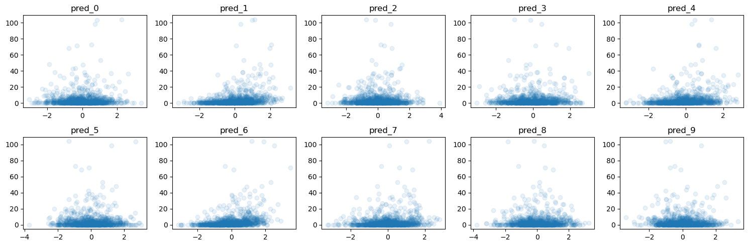
print(f"The true coefficient of the linear data generating process are:\n {true_coef}")
f = plot_y_vs_X(X_train, y_train, ncols=5, figsize=(15, 5))
The true coefficient of the linear data generating process are:
 intercept     1.000000
pred_0        0.000000
pred_1       77.903644
pred_2        0.000000
pred_3        0.000000
pred_4       63.702300
pred_5        0.000000
pred_6       95.594997
pred_7       43.869903
pred_8        0.000000
pred_9        4.118619
dtype: float64
[3]:
genuine_predictors
[3]:
intercept     1.000000
pred_1       77.903644
pred_4       63.702300
pred_6       95.594997
pred_7       43.869903
pred_9        4.118619
dtype: float64
illustrating the pipelining
[4]:
# Create a pipeline with LassoFeatureSelection and LinearRegression
pipeline = Pipeline(
[
("scaler", StandardScaler().set_output(transform="pandas")),
(
"selector",
GrootCV(
objective="poisson",
cutoff=1,
n_folds=5,
n_iter=5,
silent=True,
fastshap=True,
n_jobs=0,
),
),
("glm", PoissonRegressor()),
]
)
# Fit the pipeline to the training data
pipeline.fit(
X_train, y_train, selector__sample_weight=w_train, glm__sample_weight=w_train
)
# Make predictions on the test set
y_pred = pipeline.predict(X_test)
# Calculate the residuals
residuals = y_test - y_pred
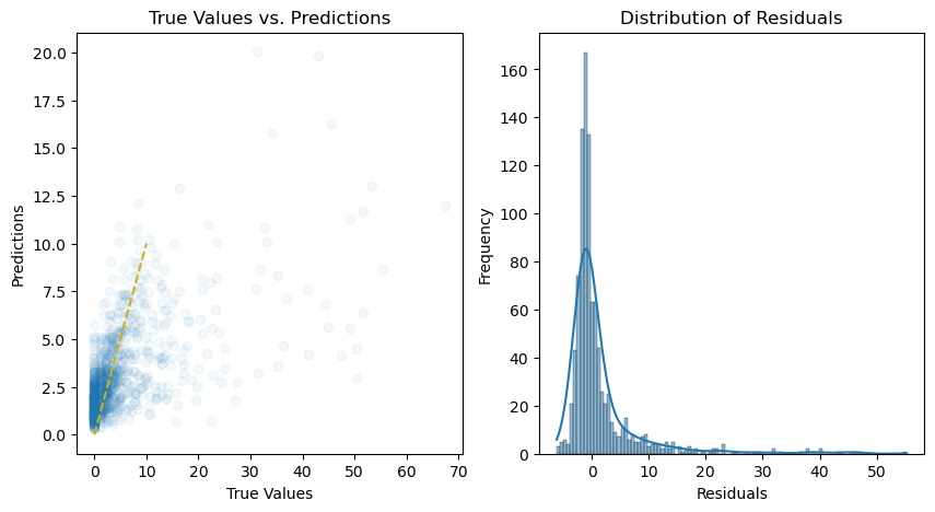
# Plot the predictions and residuals
plt.figure(figsize=(10, 5))
# Plot predictions
plt.subplot(1, 2, 1)
plt.scatter(y_test, y_pred, alpha=0.05)
plt.plot(
[min(y_test), 10],
[min(y_test), 10],
color="#d1ae11",
linestyle="--",
)
plt.xlabel("True Values")
plt.ylabel("Predictions")
plt.title("True Values vs. Predictions")
# Plot residuals
plt.subplot(1, 2, 2)
sns.histplot(residuals, kde=True)
plt.xlabel("Residuals")
plt.ylabel("Frequency")
plt.title("Distribution of Residuals")
plt.show()
use_inf_as_na option is deprecated and will be removed in a future version. Convert inf values to NaN before operating instead.
[5]:
print(
f"The selected features: {pipeline.named_steps['selector'].get_feature_names_out()}"
)
print(f"The agnostic ranking: {pipeline.named_steps['selector'].ranking_}")
print(f"The naive ranking: {pipeline.named_steps['selector'].ranking_absolutes_}")
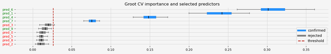
fig = pipeline.named_steps["selector"].plot_importance(n_feat_per_inch=5)
# highlight synthetic random variable
for name in true_coef.index:
if name in genuine_predictors.index:
fig = highlight_tick(figure=fig, str_match=name, color="green")
else:
fig = highlight_tick(figure=fig, str_match=name)
plt.show()
The selected features: ['pred_1' 'pred_4' 'pred_6' 'pred_7']
The agnostic ranking: [1 2 1 1 2 1 2 2 1 1]
The naive ranking: ['ShadowVar1', 'ShadowVar3', 'ShadowVar5', 'ShadowVar4', 'ShadowVar2', 'ShadowVar7', 'ShadowVar6', 'ShadowVar8', 'ShadowVar10', 'ShadowVar9']
[6]:
make_fs_summary(pipeline)
Styler.applymap has been deprecated. Use Styler.map instead.
[6]:
| predictor | scaler | selector | glm | |
|---|---|---|---|---|
| 0 | pred_0 | nan | 0 | nan |
| 1 | pred_1 | nan | 1 | nan |
| 2 | pred_2 | nan | 0 | nan |
| 3 | pred_3 | nan | 0 | nan |
| 4 | pred_4 | nan | 1 | nan |
| 5 | pred_5 | nan | 0 | nan |
| 6 | pred_6 | nan | 1 | nan |
| 7 | pred_7 | nan | 1 | nan |
| 8 | pred_8 | nan | 0 | nan |
| 9 | pred_9 | nan | 0 | nan |
Leshy#
[7]:
model = LGBMRegressor(random_state=42, verbose=-1, objective="poisson")

pipeline = Pipeline(
    [
        ("scaler", StandardScaler().set_output(transform="pandas")),
        (
            "selector",
            Leshy(
                model,
                n_estimators=20,
                verbose=1,
                max_iter=10,
                random_state=42,
                importance="fastshap",
            ),
        ),
        ("glm", PoissonRegressor()),
    ]
)

# Fit the pipeline to the training data
pipeline.fit(
    X_train, y_train, selector__sample_weight=w_train, glm__sample_weight=w_train
)

# Make predictions on the test set
y_pred = pipeline.predict(X_test)

# Calculate the residuals
residuals = y_test - y_pred

# Plot the predictions and residuals
plt.figure(figsize=(10, 5))

# Plot predictions
plt.subplot(1, 2, 1)
plt.scatter(y_test, y_pred, alpha=0.05)
plt.plot(
    [min(y_test), 10],
    [min(y_test), 10],
    color="#d1ae11",
    linestyle="--",
)
plt.xlabel("True Values")
plt.ylabel("Predictions")
plt.title("True Values vs. Predictions")


# Plot residuals
plt.subplot(1, 2, 2)
sns.histplot(residuals, kde=True)
plt.xlabel("Residuals")
plt.ylabel("Frequency")
plt.title("Distribution of Residuals")

plt.show()
Leshy finished running using native var. imp.

Iteration:      1 / 10
Confirmed:      4
Tentative:      3
Rejected:       3
All relevant predictors selected in 00:00:01.70
use_inf_as_na option is deprecated and will be removed in a future version. Convert inf values to NaN before operating instead.

[8]:
print(
f"The selected features: {pipeline.named_steps['selector'].get_feature_names_out()}"
)
print(f"The agnostic ranking: {pipeline.named_steps['selector'].ranking_}")
print(f"The naive ranking: {pipeline.named_steps['selector'].ranking_absolutes_}")
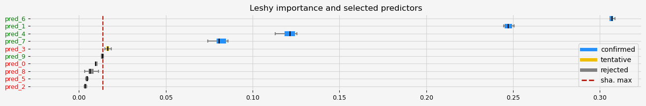
fig = pipeline.named_steps["selector"].plot_importance(n_feat_per_inch=5)
# highlight synthetic random variable
for name in true_coef.index:
if name in genuine_predictors.index:
fig = highlight_tick(figure=fig, str_match=name, color="green")
else:
fig = highlight_tick(figure=fig, str_match=name)
plt.show()
plt.show()
The selected features: ['pred_1' 'pred_4' 'pred_6' 'pred_7']
The agnostic ranking: [2 1 3 5 1 2 1 1 2 4]
The naive ranking: ['pred_6', 'pred_1', 'pred_4', 'pred_7', 'pred_0', 'pred_5', 'pred_8', 'pred_2', 'pred_9', 'pred_3']
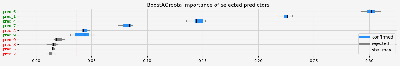
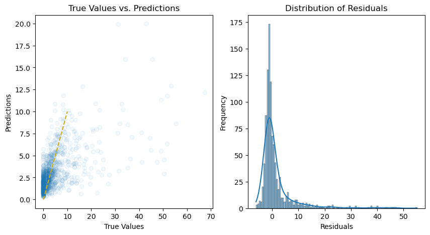
BoostAGRoota#
[9]:
model = LGBMRegressor(random_state=42, verbose=-1, objective="poisson")

pipeline = Pipeline(
    [
        ("scaler", StandardScaler().set_output(transform="pandas")),
        (
            "selector",
            BoostAGroota(
                estimator=model,
                cutoff=1,
                iters=10,
                max_rounds=10,
                delta=0.1,
                importance="fastshap",
            ),
        ),
        ("glm", PoissonRegressor()),
    ]
)

# Fit the pipeline to the training data
pipeline.fit(
    X_train, y_train, selector__sample_weight=w_train, glm__sample_weight=w_train
)

# Make predictions on the test set
y_pred = pipeline.predict(X_test)

# Calculate the residuals
residuals = y_test - y_pred

# Plot the predictions and residuals
plt.figure(figsize=(10, 5))

# Plot predictions
plt.subplot(1, 2, 1)
plt.scatter(y_test, y_pred, alpha=0.05)
plt.plot(
    [min(y_test), 10],
    [min(y_test), 10],
    color="#d1ae11",
    linestyle="--",
)
plt.xlabel("True Values")
plt.ylabel("Predictions")
plt.title("True Values vs. Predictions")

# Plot residuals
plt.subplot(1, 2, 2)
sns.histplot(residuals, kde=True)
plt.xlabel("Residuals")
plt.ylabel("Frequency")
plt.title("Distribution of Residuals")

plt.show()
use_inf_as_na option is deprecated and will be removed in a future version. Convert inf values to NaN before operating instead.

[10]:
print(
    f"The selected features: {pipeline.named_steps['selector'].get_feature_names_out()}"
)
print(f"The agnostic ranking: {pipeline.named_steps['selector'].ranking_}")
print(f"The naive ranking: {pipeline.named_steps['selector'].ranking_absolutes_}")
fig = pipeline.named_steps["selector"].plot_importance(n_feat_per_inch=5)

# highlight synthetic random variable
for name in true_coef.index:
    if name in genuine_predictors.index:
        fig = highlight_tick(figure=fig, str_match=name, color="green")
    else:
        fig = highlight_tick(figure=fig, str_match=name)

plt.show()
The selected features: ['pred_1' 'pred_4' 'pred_5' 'pred_6' 'pred_7']
The agnostic ranking: [1 2 1 1 2 2 2 2 1 1]
The naive ranking: ['pred_6', 'pred_1', 'pred_4', 'pred_7', 'pred_5', 'pred_0', 'pred_8', 'pred_9', 'pred_2', 'pred_3']
MRmr#
[11]:
mrmr = MinRedundancyMaxRelevance(
    n_features_to_select=5,
    relevance_func=None,
    redundancy_func=None,
    task="regression",  # "classification",
    denominator_func=np.mean,
    only_same_domain=False,
    return_scores=False,
    show_progress=True,
    n_jobs=-1,
)

pipeline = Pipeline(
    [
        ("selector", mrmr),
        ("scaler", StandardScaler().set_output(transform="pandas")),
        ("glm", PoissonRegressor()),
    ]
)

# Fit the pipeline to the training data
pipeline.fit(
    X_train,
    pd.Series(y_train),
    selector__sample_weight=pd.Series(w_train),
    glm__sample_weight=w_train,
)

# Make predictions on the test set
y_pred = pipeline.predict(X_test)

# Calculate the residuals
residuals = y_test - y_pred

# Plot the predictions and residuals
plt.figure(figsize=(10, 5))

# Plot predictions
plt.subplot(1, 2, 1)
plt.scatter(y_test, y_pred, alpha=0.05)
plt.plot(
    [min(y_test), 10],
    [min(y_test), 10],
    color="#d1ae11",
    linestyle="--",
)
plt.xlabel("True Values")
plt.ylabel("Predictions")
plt.title("True Values vs. Predictions")


# Plot residuals
plt.subplot(1, 2, 2)
sns.histplot(residuals, kde=True)
plt.xlabel("Residuals")
plt.ylabel("Frequency")
plt.title("Distribution of Residuals")

plt.show()
use_inf_as_na option is deprecated and will be removed in a future version. Convert inf values to NaN before operating instead.
[12]:
genuine_predictors
[12]:
intercept     1.000000
pred_1       77.903644
pred_4       63.702300
pred_6       95.594997
pred_7       43.869903
pred_9        4.118619
dtype: float64
[13]:
print(
    f"The selected features: {pipeline.named_steps['selector'].get_feature_names_out()}"
)
The selected features: ['pred_1' 'pred_3' 'pred_4' 'pred_6' 'pred_7']
[14]:
pipeline.named_steps["selector"].ranking_
[14]:
| mrmr | relevance | redundancy | |
|---|---|---|---|
| pred_6 | inf | 2.147684 | 0.000000 |
| pred_1 | 25.663894 | 1.000965 | 0.039003 |
| pred_4 | 17.704093 | 0.827022 | 0.046714 |
| pred_7 | 0.630814 | 0.044338 | 0.070287 |
| pred_3 | -11.738380 | -0.678216 | 0.057778 |