ARFS - user defined cross validation scheme - Time series applicaition

You can pass your own cross validation scheme to GrootCV. It might be useful for time series applications.

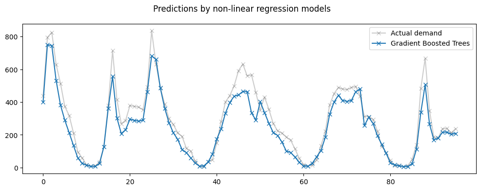
The post-selection plot below manually drops two columns and fits/predicts with that reduced frame. Selection was inspected on the full series, so the later CV numbers are exploratory. An unbiased performance comparison requires fitting selection inside each outer training window and leaving its test window untouched.

import matplotlib.pyplot as plt
import numpy as np
from sklearn.datasets import fetch_openml
from sklearn.ensemble import HistGradientBoostingRegressor
from sklearn.model_selection import TimeSeriesSplit, cross_validate

from arfs.benchmark import highlight_tick
from arfs.feature_selection.allrelevant import GrootCV

bike_sharing = fetch_openml("Bike_Sharing_Demand", version=2, as_frame=True)
df = bike_sharing.frame

y = df["count"]  # / df["count"].max()

X = df.drop("count", axis="columns")
X["weather"] = (
    X["weather"]
    .astype(object)
    .replace(to_replace="heavy_rain", value="rain")
    .astype("category")
)

import arfs

print(f"Ran with numpy {np.__version__} and ARFS {arfs.__version__}")

Ran with numpy 1.26.4 and ARFS 3.0.0

X.head()

	season	year	month	hour	holiday	weekday	workingday	weather	temp	feel_temp	humidity	windspeed
0	spring	0	1	0	False	6	False	clear	9.84	14.395	0.81	0.0
1	spring	0	1	1	False	6	False	clear	9.02	13.635	0.80	0.0
2	spring	0	1	2	False	6	False	clear	9.02	13.635	0.80	0.0
3	spring	0	1	3	False	6	False	clear	9.84	14.395	0.75	0.0
4	spring	0	1	4	False	6	False	clear	9.84	14.395	0.75	0.0

X["random_num"] = np.random.uniform(0, 1, size=len(X))

ts_cv = TimeSeriesSplit(
    n_splits=5,
    gap=48,
    max_train_size=10000,
    test_size=1000,
)

gbrt = HistGradientBoostingRegressor(
    categorical_features="from_dtype", random_state=42, loss="poisson"
)
categorical_columns = X.columns[X.dtypes == "category"]
print("Categorical features:", categorical_columns.tolist())

Categorical features: ['season', 'holiday', 'workingday', 'weather']

def evaluate(model, X, y, cv, model_prop=None, model_step=None):
    cv_results = cross_validate(
        model,
        X,
        y,
        cv=cv,
        scoring=["neg_mean_absolute_error", "neg_root_mean_squared_error"],
        return_estimator=model_prop is not None,
    )
    if model_prop is not None:
        if model_step is not None:
            values = [
                getattr(m[model_step], model_prop) for m in cv_results["estimator"]
            ]
        else:
            values = [getattr(m, model_prop) for m in cv_results["estimator"]]
        print(f"Mean model.{model_prop} = {np.mean(values)}")
    mae = -cv_results["test_neg_mean_absolute_error"]
    rmse = -cv_results["test_neg_root_mean_squared_error"]
    print(
        f"Mean Absolute Error:     {mae.mean():.3f} +/- {mae.std():.3f}\n"
        f"Root Mean Squared Error: {rmse.mean():.3f} +/- {rmse.std():.3f}"
    )


evaluate(gbrt, X, y, cv=ts_cv, model_prop="n_iter_")

Mean model.n_iter_ = 100.0
Mean Absolute Error:     42.744 +/- 1.721
Root Mean Squared Error: 67.084 +/- 3.941

all_splits = list(ts_cv.split(X, y))
train_0, test_0 = all_splits[0]

gbrt.fit(X.iloc[train_0], y.iloc[train_0])
gbrt_predictions = gbrt.predict(X.iloc[test_0])

last_hours = slice(-96, None)
fig, ax = plt.subplots(figsize=(12, 4))
fig.suptitle("Predictions by non-linear regression models")
ax.plot(
    y.iloc[test_0].values[last_hours],
    "x-",
    alpha=0.2,
    label="Actual demand",
    color="black",
)
ax.plot(
    gbrt_predictions[last_hours],
    "x-",
    label="Gradient Boosted Trees",
)
_ = ax.legend()

feat_selector = GrootCV(
    objective="poisson",
    cutoff=1,
    n_folds=5,
    folds=ts_cv,
    n_iter=5,
    silent=True,
    fastshap=False,
    n_jobs=0,
)
feat_selector.fit(X, y, sample_weight=None)
print(f"The selected features: {feat_selector.get_feature_names_out()}")
print(f"The agnostic ranking: {feat_selector.ranking_}")
print(f"The naive ranking: {feat_selector.ranking_absolutes_}")
fig = feat_selector.plot_importance(n_feat_per_inch=5)

# highlight synthetic random variable
fig = highlight_tick(figure=fig, str_match="random")
fig = highlight_tick(figure=fig, str_match="genuine", color="green")
plt.show()

Training until validation scores don't improve for 20 rounds
Early stopping, best iteration is:
[220]   training's poisson: -829.875        valid_1's poisson: -1353.86
Training until validation scores don't improve for 20 rounds
Early stopping, best iteration is:
[151]   training's poisson: -893.774        valid_1's poisson: -1404.89
Training until validation scores don't improve for 20 rounds
Early stopping, best iteration is:
[231]   training's poisson: -944.527        valid_1's poisson: -1516.04
Training until validation scores don't improve for 20 rounds
Early stopping, best iteration is:
[198]   training's poisson: -1010.91        valid_1's poisson: -1264.35
Training until validation scores don't improve for 20 rounds
Early stopping, best iteration is:
[175]   training's poisson: -1056.5 valid_1's poisson: -771.641
The selected features: ['season' 'year' 'month' 'hour' 'weekday' 'workingday' 'weather' 'temp'
 'feel_temp' 'humidity' 'windspeed']
The agnostic ranking: [2 2 2 2 1 2 2 2 2 2 2 2 1]
The naive ranking: ['ShadowVar13', 'ShadowVar10', 'ShadowVar11', 'ShadowVar9', 'ShadowVar4', 'ShadowVar6', 'ShadowVar12', 'ShadowVar3', 'ShadowVar1', 'ShadowVar8', 'ShadowVar7', 'ShadowVar2', 'ShadowVar5']

X_fs = X.drop(columns=["random_num", "holiday"])

all_splits = list(ts_cv.split(X_fs, y))
train_0, test_0 = all_splits[0]

gbrt.fit(X_fs.iloc[train_0], y.iloc[train_0])
gbrt_predictions = gbrt.predict(X_fs.iloc[test_0])

last_hours = slice(-96, None)
fig, ax = plt.subplots(figsize=(12, 4))
fig.suptitle("Predictions by non-linear regression models")
ax.plot(
    y.iloc[test_0].values[last_hours],
    "x-",
    alpha=0.2,
    label="Actual demand",
    color="black",
)
ax.plot(
    gbrt_predictions[last_hours],
    "x-",
    label="Gradient Boosted Trees",
)
_ = ax.legend()

evaluate(gbrt, X_fs, y, cv=ts_cv, model_prop="n_iter_")

Mean model.n_iter_ = 100.0
Mean Absolute Error:     41.277 +/- 2.951
Root Mean Squared Error: 64.586 +/- 5.453